mwstr_dir <- paste0(wd, "mwstr_v13/")
sql_drv <- RSQLite::SQLite()

db_m <- DBI::dbConnect(sql_drv, paste0(mwstr_dir,"mwstr_v1.3.1.gpkg"))
db_c <- DBI::dbConnect(sql_drv, paste0(mwstr_dir,"mwstr_cats_v1.3.gpkg"))
# See Appendix C.1.1 for equivalent commands to make a postgreSQL connection

r_d2ol <- terra::rast(paste0(mwstr_dir, "r_d2ol.tif"))1 Introduction
This manual describes the structure of the Melbourne Water Stream Network dataset and provides illustrations of how to extract data from the dataset. See the mwstr downloads page for access to the data, which also provides some initial guidance on handling the data. The mwstr stream explorer app provides a simple interface for extracting data from the database. This manual provides detailed advice on using the data as well as detailed descriptions of the data derivation methods.
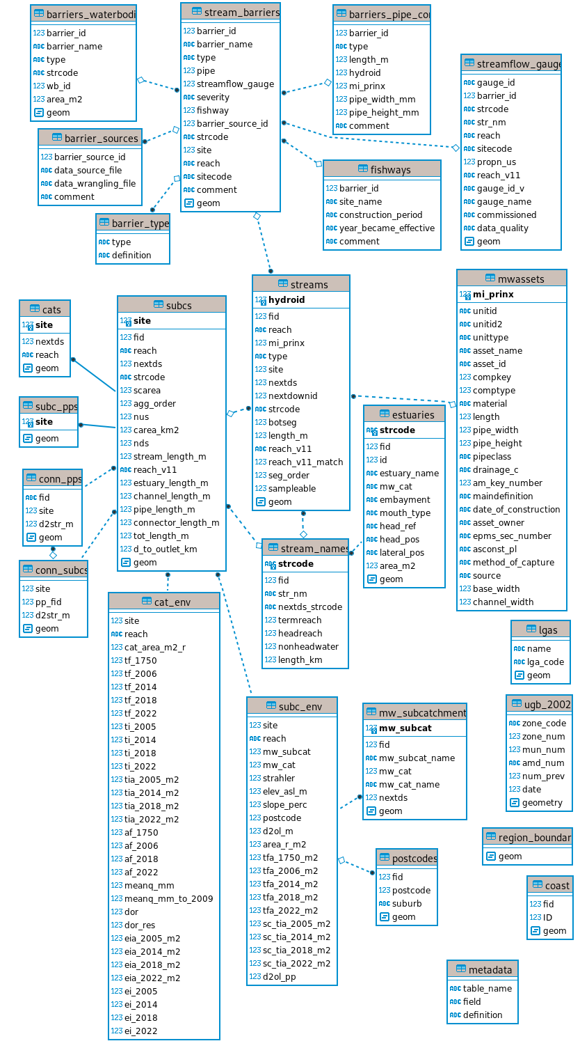
1.1 Overview of the database structure
The tables of the database and their relationships are illustrated in Figure 1.1. All but one of the vector (point, line or polygon) tables (with a geometry field) and non-spatial tables of the database are stored for download in a single geopackage file (mwstr_v1.3.1.gpkg). The cats table is large (3.3 Gb), and is supplied in its own geopackage file (mwstr_cats_v1.3.gpkg, unchanged with update of other tables to v1.3.1). Raster tables are stored for download as individual tif files. The table relationships illustrated in Figure 1.1 are derived from a PostgreSQL version of the database. Appendix C reproduces code for building a local version of a PostgreSQL database (which allows faster and more versatile access to the data than reading from the gpkg files) from the downloaded data.
The central tables of the database are: streams, which portrays the stream lines of the network (described in Chapter 2), and subcs, which portrays the subcatchment boundaries for each reach in the network (described in Chapter 3). These tables share a unique site code and a unique reach code, and the nextds (next site downstream) field in both tables permit network calculations, using the same acyclic network logic as other larger-scale, but less detailed, hydrologic datasets (Stein, Hutchinson, and Stein 2014; Linke et al. 2019). The methods used to derive the stream and subcatchment layers are described in Appendix A.
Chapter 2 of this manual describes the structure of the streams table and the smaller estuaries table.
Chapter 3 describes the structure of the subcs table and linked tables subc_pps, cats, and stream_names, as well as the DEM-derived raster tables (not shown in Figure 1.1) used to calculate catchment land use metrics. The large cats table consisting of many overlapping polygons is best accessed through SQL queries (see the mwstr downloads page).
Chapter 4 provides examples of code for mapping and analysis with the tables described in chapters 2 and 3.
Chapter 5 introduces the two primary environmental variables tables, cat_env and subc_env, and the classes of variables they hold.
Chapter 6 provides detailed information on the derivation and use of impervious cover metrics, including the tables conn_subcs and conn_pps, and the impervious raster tables (not shown in Figure 1.1) used to derive effective imperviousness.
Chapter 7 provides detailed information on the derivation and use of tree cover metrics, including the forest cover rasters (not shown in Figure 1.1) used to derive them.
Chapter 8 provides detailed information on the derivation and use of the estimate of pre-development mean annual discharge.
Chapter 9 provides detailed information on the derivation and use of the degree of regulation
metric, including the related Melbourne waterbodies database used to estimate dam volumes in each catchment.
Chapter 10 describes the derivation of the 7 stream barriers tables (top-right of Figure 1.1) and their use to derive reach-scale metrics of downstream fish barriers.
In addition to the descriptions and explanations in this manual, the metadata table defines each field in each table. All spatial tables are in the Map Grid of Australia GDA 2020 Zone 55 (crs 7855) projection. (Note that this differs from versions 1.2 and earlier of the database that were in crs 28355 [GDA 1994])
1.2 Accessing the data
The examples in this manual access the database through the program R (R Core Team 2023) using the SQLite driver through the RSQLite package (Müller et al. 2022) to connect to the geopackage files, and the terra package (Hijmans 2023) to read the raster tif files. All database files should be downloaded to a single directory to permit connection to the data. Accessing the point, line and polygon tables through a postgreSQL database is substantially faster: see Appendix C for instructions for building a local version of a PostgreSQL database from the gpkg data.
Rather than load the entire contents of the files, we create a connection to each gpkg file. The terra package takes a similar approach in opening connections to tif files. In the following examples, the gpkg and tif files of the database are in a subfolder of the working directory wd, named mwstr_v13
, thus:
Throughout this manual the object db_m signifies an active connection to the database1.
Spatial tables are opened with sf::st_read(), and non-spatial tables are opened with DBI::dbReadTable()
# Spatial tables (subcs as an example)
subcs <- sf::st_read(db_m, "subcs")
# Non-spatial tables (stream_names as an example)
stream_names <- DBI::dbReadTable(db_m, "stream_names")
Small subsets and combinations of data with SQL queries, e.g., to select just site and nextds fields of the subcs table, which can be used to rapidly calculate network relationships. By not selecting the geom field this result becomes a non-spatial table, thus:
subcs <- DBI::dbGetQuery(db_m,"SELECT site, nextds FROM subcs;")In R, this two-column table can be converted into an igraph object for rapid calculation of network relationships using the igraph package (C and Nepusz 2006) to rapidly return all upstream sitecodes from which a map of all streams the catchment can be plotted (Figure 1.2). These igraph calculations are made by the all_us() function from the file mwstr_network_functions.R (see the mwstr downloads page) to return the upstream sites, as in the sample code below (see also section 3 and section 4)2.
# find terminal reach of Gardiners Creek catchment
term_reach <- DBI::dbGetQuery(db_m,
                "SELECT termreach FROM stream_names WHERE strcode = 'GRD';")
# use all_us function (see Chapter 3) to return all upstream sites
all_sites <- all_us(term_reach, mwstr_connection = db_m)
# Use the paste (and paste0) functions to build an SQL query
all_sites_sql <- paste0("SELECT geom FROM streams WHERE site IN (",
                        paste(all_sites, collapse = ", "), ");")
# (return all_sites_sql to inspect the resulting query)
grd <- sf::st_read(db_m, query = all_sites_sql)
par(mar = c(0,0,0,0))
plot(grd)
Geopackage files can also be treated as databases in GIS software programs, and SQL queries applied in similar ways. Further examples of working with the database using SQL queries can be found in Chapters 2–5.
If the database is a PostgreSQL version,
db_mcan also contain the cats table (see Chapter 3), which is kept in a separate file in the gpkg versions, and connected via the objectdb_cin this manual.↩︎See the example code in the technical tips page of the stream network website for an example of the direct use of igraph functions for such calculations.↩︎