Melbourne Water stream network: user’s manual - 9 Degree of regulation: a flow-stress metric

9.1 Introduction

Morden et al. (2022) demonstrated that small artificial impoundments (SAIs), such as farm dams, have substantial hydrologic impacts, particularly to small, headwater streams, with potentially large impacts on stream biodiversity. They found that SAIs alter the hydrology of ~3-4 times more waterways than large impoundments in the Murrary Darling Basin. It is thus important to account for such impacts in models of ecosystem structure and function across stream networks.

Global studies of the impacts of impoundments on streams have used a “degree of regulation” index (DoR), defined as:

\[ DoR = \frac{\Sigma^n_1 V_i} {Q} \tag{9.1}\]

where V_i is the capacity of storage i of n storages upstream of a reach and Q is the mean annual discharge at the reach (Nilsson et al. 2005; Grill et al. 2014; Morden et al. 2022). These studies found DoR to be a good metric of potential biodiversity impact.

Here I document the calculation of DoR for all reaches of the stream network, and provide a summary of the spatial patterns of DoR across the region. The metrics derived in this chapter, c_dam_vol_ML_2010 (volume of dams upstream of each reach),dor_2010 (degree of regulation accounting for all upstream dams) and dor_res (accounting only for upstream reservoirs) are stored in the the cat_env table. dam_vol_ML_2010 and dor_2010 are named so because the waterbodies database from which the upstream dam data is derived is based on data collected between 2009 and 2012. dor_res is undated because the most recent reservoir was constructed pre-1980.

9.2 Methods

9.2.1 Selection of dams from the waterbodies database

I extracted SAIs and larger reservoirs (collectively called dams hereafter) from the Melbourne Water waterbodies database¹ using the wb_type field, adjusting for various errors detected during the selection process. Our primary aim was to identify constructed dams used at least to some extent for extraction of water for agricultural or other human use. Values of type ‘dam’,‘farm dam’,‘farm pond’, ‘rural storage’,‘town rural storage’, ‘rural irrigation storage’,‘rural licensed storage’,‘water storage’, and ‘reservoir’ (all converted to lower case) were selected. This selection thus omitted natural waterbodies, artificial waterbodies with no connection to natural drainage (eg sewerage ponds, etc.), and stormwater treatment wetlands from which no water is harvested.

Some of the initially selected waterbodies were removed or adjusted during the subsequent process. Most of those changes, which were the result of errors in the waterbodies database will not be necessary with future, corrected versions of the waterbodies database. For other subsequent exclusions, see below.

The mwb database is a highly accurate record of waterbodies across the region, but its classification of dams versus other waterbody types is not perfect. The barriers analysis Chapter 10 provided a dataset of online dams that had been collected independently from the mwb compilation. In cross-checking the two datasets, 6% of the dams in the barriers dataset had not been identified as dams in the mwb dataset. Following manual corrections during this work, it is likely that the mwb database correclty classifies ~95% of SAIs in the region. Given that most of the missed dams will be small, the resulting understimation of DoR in this work is likely to be substantially less than 5%.

9.2.2 Allocation of dam outlets to stream network subcatchments

DoR calculation requires that the outlet of each dam is allocated to a subcatchment in the stream network. The waterbodies catchments data in the waterbodies database used waterbody outlets that were in some cases incorrect, and the outlets were not saved as a point dataset, making allocation of every waterbody to a subcatchment more difficult. It was thus necessary to first allocate each dam to its correct subcatchment. Subsidiary benefits of the exercise include:

Identification of on-line and off-line dams;
Validation and correction of catchment boundaries and areas of on-line dams in the waterbodies database;
Identification of problematic inconsistencies between the stream network and waterbodies data (for instance where wetlands span adjacent stream catchments, or wetlands that fall outside stream network catchments);
Identification of incorrectly classed waterbodies;
Identification of stream lines passing through waterbodies that had not been previously been identified as ‘connecting lines through waterbodies’;
A partial set of outlet points (for online dams only);
A workflow that can be replicated for non-dam waterbodies.

The code used to achieve the above aims (in the source code of this document) used the following logic:

Dams (in the wbs_dams table) were separated into four groups: combinations of a) online (those intersecting a stream line) and offline, and b) those that sit within a single stream network subcatchment (single) and those that span multiple subcatchments (multi). This process also revealed 607 dams that fall outside the stream network subcatchments, which were not considered further.
Offline-single dams were associated with the subcatchment (reach and site fields in the stream network database) in which they lie.
Online-single dams were associated with the subcatchment in which they lie. For all online dams (both single and multi), two new tables were created: a table of linestrings recording all stream lines flowing through the wetland; and a table of points recording the wetland outlet (the bottom point of the most downstream stream line passing through the wetland).
Offline-multi dams were associated with the subcatchment that intersected with the majority of the wetland area.
Online-multi dams were associated with the most downstream point on the stream lines that intersected the waterbody polygon, which was assumed to be the outlet of the dam. In some cases, because of inconsistencies between the waterbodies and the streams layers, there were two most downstream points on independent streamlines, upstream of a confluence. In those cases, a point near the most upstream end of the stream line downstream of the confluence was selected as the outlet.

Derivation of online-multi dam outlets revealed a small number of network errors in the stream database, corrected in version 1.3.

For online dams, the inferred outlet location was recorded in a spatial table which recorded the stream network reach on which it sits, the proportion of reach length upstream on which it sits, and the resulting sitecode (using the sitecode convention of Walsh 2023). This table was used to recalculate the catchment boundaries for online dams in the waterbodies database.

For all dams, two additional tables were created:

a subsetted version of the waterbodies table that included the stream network ‘reach’ and ‘site’ codes, a comment identifying the online/offline, single/multi status of each wetland and the inferred dam volume (see below);
a spatial table of the intersection of stream lines and dams , the stream line passing through each dam, clipped to the dam polygon. This table was used to recalculate the total length of streams that passes through a waterbody in the stream network layer (see below). The streams table contains a type of line “connecting line through waterbody”, but such lines have only been drawn through large waterbodies, and not many smaller dams. Using this set of lines provided a more realistic estimate of the full length of streams inundated by dams in the region. These estimates have not been included in the mwstr database.

9.2.3 Estimation of dam volume and DoR.

For waterbodies listed as reservoirs I extracted capacities from ANCOLD (Australian National Committee on Large Dams Incorporated) (2010) and from the Victorian Government dams database https://www.water.vic.gov.au/managing-dams-and-water-emergencies/dams. For all dams not registered in either of those sources, I estimated dam volume (V in ML) after Morden et al. (2022) using the equation of Fowler et al. (2015):

\[ V = 0.0001042 \cdot A^{1.3213} \tag{9.2}\]

where A is the surface area of the dam in m².

To calculate DoR (Equation 9.1) for each reach in the stream network, I summed the volumes of all dams in the catchment upstream of (and including) the reach, and divided it by the estimated mean annual discharge of the reach in ML. Mean annual discharge depth (in mm) for each reach was estimated from the Australian Bureau of Meteorology gridded runoff data, derived from the Australian Landscape Water Balance AWRA-L Model data (see https://github.com/cjbwalsh/mwstr/env_q_compilation.R). This was converted to discharge in ML by multiplying by the catchment area in km².

Morden et al. (2022) excluded large impoundments that were off-stream storages whose primary source of water was extraction from another storage or waterway, rather than runoff from their immediate upstream watershed. Following this logic, I excluded service reservoirs with no catchment area (roofed or open tanks: three Western Water tanks—which were the only waterbodies with type ‘Water Storage`—Dromana, Moorabbin, Somerton and Mornington Reservoirs). It is possible that some of the 1,710 waterbodies classes as ’Town rural storage’ should be excluded for the same reason, but the ~6 of these that I checked were all dams receiving runoff from their own catchments.

However, I took a different approach for the large service reservoirs of the Melbourne region. While Silvan², Cardinia, Sugarloaf, YanYean, and Greenvale reservoirs are primarily filled by water imported from other catchments or sources (i.e. the desalination plant), their outlets all lie on a stream line and they receive water from their own catchments. As the only flows to the streams at their outlets (if any) are environmental flow releases, and none of them spill (or do so only extremely rarely), I set DoR at their outlets to 1. Similarly, Upper Yarra and Maroondah Reservoirs never or rarely spill because their effective capacities are increased by diverting much of their inflows to the above storage reservoirs. I also set DoR for those two reservoirs to 1, by making their volumes equivalent to the mean annual discharge at their outlet (without that adjustment, their DoR was 0.89 and 0.42, respectively).

In addition, the registered volumes of Beaconsfield and Orde Hill/Wilmigongon Reservoirs, which were represented by two polygons, were assumed to apply to both polygons, so the volume of the smaller polygon in both cases was set to zero.

9.3 Results

Figure 9.1: Relationship between reservoir volumes extracted from ANCOLD or DWELP databases and estimates of volume using Equation 9.2 from Fowler et al. (2015). The dotted line indicates a 1:1 relationship.

Figure 9.1 provides an initial confirmation that the equation for estimating dam volume of Fowler et al. (2015) is appropriate for the Melbourne Water region, by comparing estimated volumes with the registered volumes of the region’s reservoirs. The relationship is close to 1:1 (slope = 1.02), with an R² (when both values are log-transformed) of 0.96, which is similar to the relationship reported by Fowler et al. (2015) for the data from which they derived the equation.

Table 9.1: Summary of lengths of stream (those large enough for macroinvertebrates to be sampled [sampleable] and all streams) downstream of any dam, and downstream of reservoirs, and length of stream submerged by dams and reservoirs. The submerged lengths are not included (nor piped sections) in the calculations of total stream length or stream lengths downstream.
Class	Sampleable	All
Total length (km)	8,053	24,829
Length downstream of any dam (km)	6,604	13,833
Length downstream of any dam (%)	82	56
Length downstream of reservoirs (km)	1,081	1,083
Length downstream of reservoirs (%)	13	4
Length downstream of any dam, DoR > 0.167 (km)	2,037	4,270
Length downstream of any dam, DoR > 0.167 (%)	25	17
Length downstream of reservoirs, DoR > 0.167 (km)	734	736
Length downstream of reservoirs, DoR > 0.167 (%)	9	3
Length submerged by dams (km)		1,042
Length submerged by reservoirs (km)		20

The total volume of SAIs in the Melbourne region (136 GL), is small compared to the total volume of reservoirs (888 GL). However, only 4% of stream length across the region is downstream of reservoirs, while 56% of stream length is downstream of any dam (Table 9.1). If only streams large enough to be sampled for macroinvertebrates are considered, 13% are downstream of reservoirs, while 82% are downstream of any dam. Morden et al. (2022) tentatively adoped DoR = 0.167 (i.e. storage upstream greater than 16.7% of their annual discharge) as a threshold above which rivers are likely to be impacted by flow stress (noting that such a threshold requires validation). While two-thirds of the 1,083 km of stream downstream of reservoirs have DoR > 0.167, only about one-third of the 13,833 km of stream downstream of any dam have such a high level of regulation impact (Table 9.1).

Over 1000 km of stream has been inundated under on-line dams. Only a small proportion of this submerged length is under reservoirs (Table 9.1).

The degree of regulation tends to be greatest in the drier streams of the west, and in small streams in the north of Westernport (Figure 9.2, Figure 9.3,Figure 9.4).

Figure 9.2: All streams, channels, pipes and estuaries and of the region shaded by degree of regulation (DoR, variable dor_2010 in the cat_env table of the database). The colour scheme was chosen to distinguish reaches unlikely to be impacted by flow stress (DoR < 0.1) and those likely to be (DoR > 0.167). These thresholds are based on the range of thresholds identified from the literature by Morden et al. 2022.

Figure 9.3: All streams of the region large enough to sample macroinvertebrates using standard methods shaded by degree of regulation (DoR, variable dor_2010 in the cat_env table of the database). See Figure 9.2 for an explanation of the chosen colour scheme.

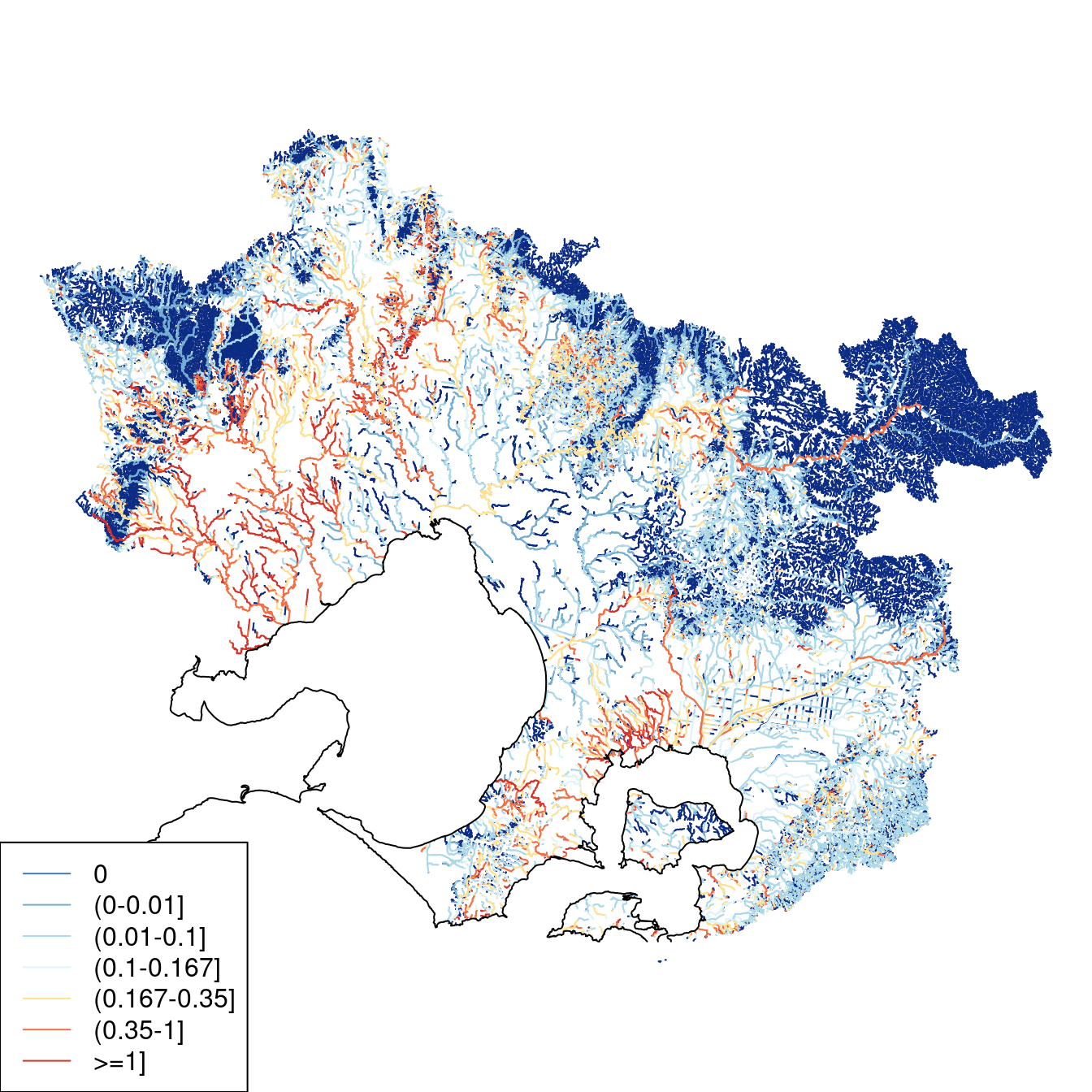
Figure 9.4: All streams of the region large enough to sample macroinvertebrates using standard methods shaded by degree of regulation (DoR) calculated only for waterbodies classed as ‘Reservoir’ (variable dor_res). See Figure 9.2 for an explanation of the chosen colour scheme.

9.4 Discussion

If DoR >0.167 is considered a level above which stream hydrology is significantly altered, then SAIs alter ~3 times the length of ‘sampleable’ stream than reservoirs in the Melbourne region (Table 9.1), which is consistent with the finding of Morden et al. (2022) for the Murray-Darling basin.

This version of DoR should be considered preliminary, as further refinements could be applied following review. Questions to be considered in review include:

Can DoR be improved by including estimation of abstraction from each dam?
Is there sufficient, reliable data to make such an estimate reliable?
How can environmental flow releases be incorporated into DoR, or should these be captured in a separate index to permit separate estimation of degrading impact of dams and restorative impact of environmental flows?
Is the inclusion of dams where the average slope of the surrounding terrain was < 0.25% appropriate? Morden et al. (2022) argued that: “in such areas, surface runoff is very unlikely to reach a waterway under natural circumstances, and so while small impoundments here may have substantial biodiversity value, they were assumed to have no direct hydrological impact on downstream waterways”.