5 Reach and catchment environmental metrics
I have calculated many environmental metrics for all reaches of the stream network. These metrics have many potential uses for stream management and research. The remaining chapters of this manual describe the derivation of the metrics and the structure of the tables holding them.
Two primary environmental metric tables hold the most commonly used metrics:
Table cat_env contains environmental variables for every reach that describe catchment attributes.
Table subc_env contains environmental variables for every reach that describe attributes of the reach or its immediate subcatchment.
The two tables contain site and reach fields matching those fields in the subcs table. The tables are broadly separated into variables that describe the reach or its local subcatchment (subc_env) and those that describe the catchment upstream of the reach (cat_env). Metrics fall into the following classes (some of which have fields in both subc_env and cat_env.). See Figure 1.1 for the full list of fields in these two tables.
There are two almost identical versions of subcatchment (and catchment) area (in m2) in the database. area_r_m2 in the subc_env table is the sum of gridcell areas for each subcatchment in the r_site raster table. scarea in the subcs table is the area of the polygons in the table. They differ because a small number of subcatchment polygons were manually altered to correct network relationships, resulting in an imperfect match with the DEM gridcells on which the subcatchments were originally calculated. scarea is a more accurate estimate of subcatchment area, but area_r_m2 was used for calculating subcatchment statistics (e.g. impervious cover and tree cover fractions) from raster data. cat_area_m2_r in the cat_env table sums area_r_m2 for all upstream subcatchments, and carea_km2 in the subcs table similarly sums and converts to km2 scarea.
5.1 Impervious cover
Impervious area as a fraction of the upstream catchment (total imperviousness, TI) is a primary measure of urban density. Effective imperviousness (EI) is an important measure of urban stormwater drainage impacts (Walsh et al. 2022). I have calculated these metrics for 2005, 2018, and 2022 (with 2012 and 204 to follow). The fields ti_XXXX and ei_XXXX in the cat_env table record these two metrics for year XXXX. The fields tia_XXXX_m2 and eia_XXXX_m2 in the subc_env table record the total and effect area of impervious surfaces in m2 within each subcatchment. See Chapter 6 for full details.
5.2 Tree canopy cover
Tree canopy cover near streams is a strong predictor of in-stream biotic assemblages (Peterson et al. 2010; Walsh and Webb 2014), and catchment tree canopy cover is an important predictor of streamflow volumes (Zhang, Dawes, and Walker 2001). I thus calculated both tree canopy area as a fraction of stream catchment (TF), and tree canopy area weighted by flow distance to and along streams as a fraction of similarly weighted catchment area (Attenuated forest cover, AF). I have calculated these metrics for 1750 (estimated from ecological vegetation classes), 2006, 2018 and 2022. TF and AF are recorded as fields tf_XXXX and af_XXXX in the cat_env table, for the year XXXX. Total area of tree canopy cover in each subcatchment in m2, tfa_XXXX_m2, is recorded in the subc_env table. See Chapter 7 for full details, and Appendix E for a description of quality control and assessment of the 2018 and 2022 data.
5.3 Flow
Two estimates of mean annual runoff were calculated: for the period 1911-2022, and 1911-2009 for equivalence with the measure of mean discharge used in earlier studies of the region. These were recorded as fields meanq_mm and meanq_mm_to_2009, respectively, in the cat_env table. See Chapter 8 for full details.
5.4 Flow stress: degree of regulation
A degree of regulation
index (DoR) was calculated as a measure of flow stress. It is the ratio of the volume of dams in the catchment to mean annual discharge volume (Morden et al. 2022). The dam volumes, derived from the Melbourne Water waterbodies database, collected between 2009 and 2012, was recorded as the field, c_vol_dams_megalitre_2010 in the cat_env table. Also in that table, DoR counting all dams was recorded as dor_2010, and counting only large reservoirs (which all pre-date 2010 by many years) as dor_res. See Chapter 9 for full details.
5.5 Barriers to fish passage
Barriers to fish (and potentially other fauna) migration such as weirs, dams, and piped streams can limit the distributions of species. The number of barriers to instream migration downstream of each reach was calculated from a revised dataset of barriers that is included in the database. I calculated two variants—number of partial barriers downstream and number of full barriers downstream, for 1996 and 2023. These are recorded in the subc_env table as fields n_part_barriers_ds_XXXX, and n_full_barriers_ds_XXXX, respectively, with XXXX signifying the year. The function recalc_barriers() in the script mwstr_network_functions allows rapid calculation of these variables for any year between 1996 and 2023. See Chapter 10 for full details.
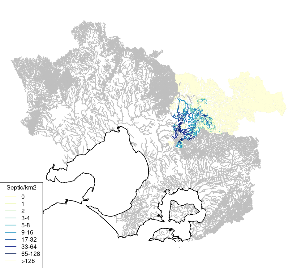
5.6 Septic tank density
Septic tanks can be major contributors to nitrogen export from catchments (Bernhardt et al. 2008), and their density is a strong predictor of nitrogen concentrations in Melbourne’s streams (Walsh and Kunapo 2009). Sewer backlog programs around peri-urban Melbourne are aiming to replace septic systems with reticulated sewerage (Victorian Auditor-General’s Office 2006), but septic tanks are common throughout the region, even in some areas with reticulated sewerage.
I calculated catchment septic tank density (sep_per_km2) for a portion of the region and added to the cat_env table. Data were only available for the Yarra Ranges Council area (data source: Yarra Ranges Council from around the year 2000), with a small amount of further data for the Dobsons Creek catchment (data source: Yarra Valley Water 2017), and augmented estimates for parts of the Menzies Creek catchment that fall outside the Yarra Ranges Council (Figure 5.1).
5.7 Catchment geology
Many measures of catchment geology or soil type are possible, using Government spatial data such as the Geomorphological map units of Victoria (Rees et al. 2017) and Victorian Soil type mapping (Anon. 2018). Rather than generate a large number of geological or soil metrics, I calculated two example metrics from the geormophological map: proportion of catchment area with basalt geology (c_basalt), and granitic geology (c_granitic), both in the cat_env table, and provide the code I used to calculate them as a template for other similar calculations (including any polygon land-cover data for the region). The resulting distributions of catchment geology are show in Figure 5.2.
# GMU250.shp downloaded from data.vic.gov.au and stored in geol_dir
# db_m is a connection to the database as in section 1.2
system.time({
geol <- terra::vect(paste0(geol_dir,"GMU250.shp"))
geol <- terra::project(geol, "epsg:7855")
geol <- terra::makeValid(geol)
# unique(geol$LITHOLOGY) #15 classes including NAs...
# sum(is.na(geol$LITHOLOGY))  #12 - all in MW region are waterbodies, so..
geol$LITHOLOGY[is.na(geol$LITHOLOGY)]<-'Water Body'
# combine...
geol$LITHOLOGY[grep('Granite|Granitic',geol$LITHOLOGY)]<-'Granitic'
geol$LITHOLOGY[grep('Basalt|Volcanics',geol$LITHOLOGY)]<-'Basalt'
lith_groups <- unique(geol$LITHOLOGY)
geol$lith_id <- match(geol$LITHOLOGY,lith_groups) # Basalt = 1; Granitic = 5.
r_site <- terra::rast("directory_of_choice/mwstr_v13/r_site.tif")
geol_r <- terra::rasterize(geol, r_site, field = "lith_id") # ~ 10 s
}) # ~30 s
#### Note the next zonal calculations require ~ 70 Gb RAM
system.time({
basalt_site <- terra::zonal(geol_r, r_site,
                          fun = function(x){sum(x == 1, na.rm = TRUE)})
}) # ~ 4.5 min
gc()
system.time({
granite_site <- terra::zonal(geol_r, r_site,
                          fun = function(x){sum(x == 5, na.rm = TRUE)}) # ~ 4.5 min
})
gc()
# Assume an active connection to mwstr called db_m
subcs_geol <- DBI::dbGetQuery(db_m,
          paste0("SELECT subcs.site, subcs.nextds, subcs.nus, ",
                 "subcs.agg_order,subcs.scarea, cat_env.cat_area_m2_r ",
                 "FROM subcs JOIN cat_env ON subcs.site = cat_env.site;"))
DBI::dbDisconnect(db_m)
system.time({
subcs_geol <- subcs_geol[order(subcs_geol$nus, subcs_geol$agg_order),]
subcs_geol$sc_basalt <-
  basalt_site$lith_id[match(subcs_geol$site, basalt_site$site)]
subcs_geol$sc_granite <-
  granite_site$lith_id[match(subcs_geol$site, basalt_site$site)]
subcs_geol$c_granite <- subcs_geol$c_basalt <- NA
# All subcatchments of agg_order 1 have no subcatchments upstream. Their
# catchment area (in km2) = their subcatchment area (in m2 * 1e-6)
subcs_geol$c_basalt[subcs_geol$agg_order == 1] <-
  subcs_geol$sc_basalt[subcs_geol$agg_order == 1]
subcs_geol$c_granite[subcs_geol$agg_order == 1] <-
  subcs_geol$sc_granite[subcs_geol$agg_order == 1]
  for(i in min(which(subcs_geol$agg_order == 2)):nrow(subcs_geol)){
# Loop through all remaining subcatchments, adding its subcatchment area to the
# (already calculated) catchment areas of subcatchments immediately upstream
    subcs_geol$c_basalt[i] <-
      sum(subcs_geol$c_basalt[subcs_geol$nextds == subcs_geol$site[i]],
          subcs_geol$sc_basalt[i])
    subcs_geol$c_granite[i] <-
      sum(subcs_geol$c_granite[subcs_geol$nextds == subcs_geol$site[i]],
          subcs_geol$sc_granite[i])
    if(i %% 10000 == 0) cat(i,"\n")
  }
}) # 1.5 min
# multiply by 25 because each gridcell is 25 m2
subcs_geol$c_granite <- subcs_geol$c_granite*25/subcs_geol$cat_area_m2_r
subcs_geol$c_basalt <- subcs_geol$c_basalt*25/subcs_geol$cat_area_m2_r
5.8 Air temperature
Mean daily air temperature at a reach is a strong predictor of mean daily stream temperature. While the diel range of air temperature is greater than stream water, temperature of both air and water tend to vary around a similar value given equivalent shading. Other factors such as shading by tree cover, slope, aspect, flow volume, and groundwater, stormwater and industrial inputs can influence stream temperature. But mean daily air temperature provides a good measure of stream temperature in the absence of anthropogenic alterations to effects such as tree cover, stormwater drainage and flow modification. It also has the advantage of being compatible with a measure by which climate-warming predictions are communicated.
Like geological variables, there are many possible temperature metrics that could be calculated for the network. Unlike the geological data, the source data from the the Australian Bureau of Meteorology Australian Gridded Climate Data (AGCD: Australian Bureau of Meteorology, n.d.) is raster-based. I thus provide the code I used to calculate mean temperature, which can be used as a template for calculating other metrics.
The following code requires specification of a directory grid_dir used to store the rasters, and a connection to the mwstr database, db_m.
# 1. Download all available AGCD data (daily maximum tmax and minimum tmin)
#    Each .nc file is a stack of 365/6 daily rasters for a year.
for(i in 1910:2022){
download.file(paste0("https://thredds.nci.org.au/thredds/fileServer/zv2/agcd/",
                     "v1-0-1/tmax/mean/r005/01day/agcd_v1-0-1_tmax_mean_r005_daily_",
                     i, ".nc"),
              paste0(grid_dir, "tmax/agcd_v1-0-1_tmax_mean_r005_daily_",i, ".nc"))
download.file(paste0("https://thredds.nci.org.au/thredds/fileServer/zv2/agcd/",
                     "v1-0-1/tmin/mean/r005/01day/agcd_v1-0-1_tmin_mean_r005_daily_",
                     i, ".nc"),
              paste0(grid_dir, "tmin/agcd_v1-0-1_tmin_mean_r005_daily_",i,".nc"))
}

# 2. a) Crop each raster stack to the mwstr region,
#    b) calculate the mean daily maximum and mean for each year
#    c) and add to a stack of 131 rasters of annual means,
#       (one raster for each year)
region <- sf::st_read(mwstr, "region_boundary")
region <- sf::st_transform(region, crs = 4326)
mw_ext <- terra::ext(region)

system.time({
for(i in 1910:2022){
    tmini <- terra::rast(paste0(grid_dir, "tmin/agcd_v1-0-1_tmin_mean_r005_daily_",i,".nc"))
    tmini <- terra::crop(tmini,mw_ext)
    tmaxi <- terra::rast(paste0(grid_dir, "tmax/agcd_v1-0-1_tmax_mean_r005_daily_",i,".nc"))
    tmaxi <- terra::crop(tmaxi,mw_ext)
    if(i == 1910){
      mw_mean_max_annual_grid <- terra::mean(tmaxi)
      mw_mean_min_annual_grid <- terra::mean(tmini)
# At this stage, seasonal means could be calculated by subsetting, e.g:
#    mw_mean_max_summer_grid <- mean(subset(xi,c(1:60,335:dim(xi)[3])))
    }else{
      mw_mean_max_annual_grid <- c(mw_mean_max_annual_grid,
                                   terra::mean(tmaxi))
      mw_mean_min_annual_grid <- c(mw_mean_min_annual_grid,
                                   terra::mean(tmini))
    }
    cat(i,"\n")
  }
})  # 24 min
names(mw_mean_max_annual_grid) <- 1910:2022
names(mw_mean_min_annual_grid) <- 1910:2022
# 3. Estimate the annual means of daily mean temperature as mean of min and max
x <- terra::sds(list(r_tmin_ann, r_tmax_ann))
r_tmean_ann <- terra::app(x, mean)
# 4. Calculate long-term mean raster using the full record of 113 years
r_meant <- terra::mean(r_tmean_ann, na.rm = TRUE)
# 5. calculate 30-year means:
# a) set indices
y30_1950 <- which(names(r_tmean_ann) %in% 1921:1950)
y30_1980 <- which(names(r_tmean_ann) %in% 1951:1980)
y30_2010 <- which(names(r_tmean_ann) %in% 1981:2010)
y30_2022 <- which(names(r_tmean_ann) %in% 1993:2022)
# b) calculate 30-y mean rasters
r_y30_1950 <- terra::sds(list(r_tmin_ann[[y30_1950]], r_tmax_ann[[y30_1950]]))
r_tmean_y30_1950 <- terra::app(r_y30_1950, mean)
r_meant_y30_1950 <- terra::mean(r_tmean_y30_1950, na.rm = TRUE)
r_y30_1980 <- terra::sds(list(r_tmin_ann[[y30_1980]], r_tmax_ann[[y30_1980]]))
r_tmean_y30_1980 <- terra::app(r_y30_1980, mean)
r_meant_y30_1980 <- terra::mean(r_tmean_y30_1980, na.rm = TRUE)
r_y30_2010 <- terra::sds(list(r_tmin_ann[[y30_2010]], r_tmax_ann[[y30_2010]]))
r_tmean_y30_2010 <- terra::app(r_y30_2010, mean)
r_meant_y30_2010 <- terra::mean(r_tmean_y30_2010, na.rm = TRUE)
r_y30_2022 <- terra::sds(list(r_tmin_ann[[y30_2022]], r_tmax_ann[[y30_2022]]))
r_tmean_y30_2022 <- terra::app(r_y30_2022, mean)
r_meant_y30_2022 <- terra::mean(r_tmean_y30_2022, na.rm = TRUE)
# # (Inspect a raster, adding the coastline for orientation)
# terra::plot(r_meant_y30_2022)
# coast <- sf::st_read(db_m, "coast")
# coast <- terra::vect(sf::st_transform(coast, crs = 4326))
# terra::plot(coast, add = TRUE)
# 6. extract the 30-year mean values for every subc pourpoint
rmeant_30y <- c(r_meant_y30_1950,r_meant_y30_1980,
r_meant_y30_2010,r_meant_y30_2022)
names(rmeant_30y) <- paste0("meant_y30_",c(1950,1980,2010,2022))
subc_pps <- sf::st_read(db_m, 'subc_pps')
subc_pps <- sf::st_transform(subc_pps, crs = 4326)
subc_pps <- terra::vect(subc_pps)
x <- suppressWarnings(terra::extract(rmeant_30y, subc_pps))
x <- data.frame(site = subc_pps$site, x[,-1])The above code calculates the mean daily air temperature at the pour-point (lowest point) of each subcatchment in the network as the mean of the minimum and maximum daily temperature grids from the AGCD (Australian Bureau of Meteorology, n.d.), for four 30-year periods: to 1950, 1980, 2010 and 2022.
Across the region, mean temperatures during each of these periods were highly correlated, but warming of ~1 C\(^\circ\) over the century is evident (Figure 5.3).

The four means are recored in the subc_env table as meant_y30_1950, meant_y30_1980 meant_y30_2010, and meant_y30_2022. Figure 5.4 shows the distribution of the last of these among sampleable
streams using the following code.
# db_m is a connection to the database as in section 1.2
streams <- sf::st_read(db_m,
                       query = "SELECT * FROM streams WHERE sampleable = 1;")
airtemp <- DBI::dbGetQuery(db_m, "SELECT site, meant_y30_2022 FROM subc_env;")
streams$meant_y30_2022 <-
  airtemp$meant_y30_2022[match(streams$site, airtemp$site)]
plot(streams["meant_y30_2022"])
5.9 Elevation, slope and aspect
I calculated elevation (above sea-level in m, subc_env.elev_asl_m, Figure 5.5 A) and slope (percentage, subc_env.slope_perc, Figure 5.5 B) from the filled 5-m digital elevation model (table r_dem). I calculated aspect (as northness, Figure 5.5 C) from the stream lines. These three reach attributes are stored in the subc_env table.
The lines in the streams table are accurately delineated throughout the region, having been derived from a 1-m-resolution DEM, and a more accurate estimate of slope could be achieved using them than flow distances from the 5-m DEM. I took a hybrid approach to estimating slope of each reach by calculating the difference in elevation between the 5-m raster pourpoints for each subcatchment and its upstream subcatchment(s), and used the length of the stream line through the subcatchment as the horizontal distance.
Slope was calculated as a percentage as:
\[ 100 \cdot \frac{\Delta E}{\sqrt{{L}^2 + {\Delta E}^2}} \tag{5.1}\]
where \(\Delta E\) = the difference in elevation between upstream and downstream points and \(L\) is the total length of the stream lines (of all types) in the reach. Slopes were not calculated for headwater reaches, most of which were very short line segments. Negative slopes, of which there were 1672, almost all very small, were set to zero.
Aspect can influence how shaded a reach is with a reach flowing north-south likely to be less shaded by its banks and hillslopes than a reach flowing east-west. A more complete measure of such an effect could integrate shading calculated from a DEM and daily patterns of solar radiation, but northness is offered as an initial approximation. Northness was calculated from the angle between the most downstream and most upstream points of the line(s) of each reach. It was calculated as
\[ abs(cos(\theta)) \tag{5.2}\]
where \(\theta\) is the angle in radians from North between the two points. Thus for a reach flowing north to south (or vice-versa) northness = 1, and for a reach flowing east to west (or vice versa) northness = 0.
# db_m is a connection to the database as in section 1.2
str_slope_elev <- sf::st_read(db_m, query =
    "SELECT streams.geom, subc_env.elev_asl_m, subc_env.slope_perc,
     subc_env.northness, streams.reach, streams.sampleable, subcs.agg_order
      FROM streams JOIN subc_env ON streams.site = subc_env.site
      JOIN subcs on subc_env.site = subcs.site;")
# Order by agg_order to place largest streams on top of plot
str_slope_elev <- str_slope_elev[order(str_slope_elev$agg_order),]
# Set colors for maps
str_slope_elev$elev_class <-
  as.numeric(cut(str_slope_elev$elev_asl_m,
                 breaks = c(-10,10,20,40,80,160,320,640,1340)))
str_slope_elev$elev_col <-
  RColorBrewer::brewer.pal(8,"Spectral")[match(str_slope_elev$elev_class,1:8)]
str_slope_elev$slope_class <-
  as.numeric(cut(str_slope_elev$slope_perc, breaks = c(0,1,2,4,8,16,32,75)))
str_slope_elev$slope_col <-
  RColorBrewer::brewer.pal(7,"Spectral")[match(str_slope_elev$slope_class,1:7)]
str_slope_elev$north_class <-
  as.numeric(cut(str_slope_elev$northness,
                 breaks = c(-0.1,0.2,0.4,0.6,0.8,1.1)))
str_slope_elev$north_col <-
  RColorBrewer::brewer.pal(5,"Spectral")[match(str_slope_elev$north_class,1:5)]
# Plot maps
par(mfrow = c(2,2), mar = c(0,0,0,0))
plot(str_slope_elev$geom, col = str_slope_elev$elev_col)
title(main = "A.", adj = 0, line = -1)
legend("bottomleft", lty = 1, col = RColorBrewer::brewer.pal(8, "Spectral"),
  legend = c("<10","10-20","20-40","40-80","80-160","160-320","320-640",">640"),
  cex = 0.7, title = "Elevation (m)")
plot(str_slope_elev$geom, col = str_slope_elev$slope_col)
title(main = "B.", adj = 0, line = -1)
legend("bottomleft", lty = 1, col = RColorBrewer::brewer.pal(7, "Spectral"),
  legend = c("<1","1-2","2-4","4-8","8-16","16-32",">32"),
  cex = 0.7, title = "Slope (%)")
plot(str_slope_elev$geom, col = str_slope_elev$north_col)
title(main = "C.", adj = 0, line = -1)
legend("bottomleft", lty = 1, col = RColorBrewer::brewer.pal(5, "Spectral"),
  legend = c("0-0.2","0.2-0.4","0.4-0.6","0.6-0.8","0.8-1,0"),
  cex = 0.7, title = "Northness")
5.10 Strahler stream order
I calculated Strahler order (variable strahler in subc_env, a numerical measure of branching complexity) for the reaches of the network using the following code, which applies the algorithm described at https://en.wikipedia.org/wiki/Strahler_number.
subcs_s <- subcs[c("site","nextds","nus","agg_order")]
subcs_s <- subcs_s[order(subcs_s$nus, subcs$agg_order),]
subcs_s$strahler <- NA
subcs_s$strahler[subcs_s$nus %in% c(0)] <- 1
# If there are no upstream lines strahler = 1
  for(i in min(which(is.na(subcs_s$strahler))):dim(subcs_s)[1]){
    if(sum(subcs_s$nextds == subcs_s$site[i]) == 1){
# If the site is a split in a stream line not at a confluence make strahler the
# value of the site upstream
      subcs_s$strahler[i] <- subcs_s$strahler[subcs_s$nextds == subcs_s$site[i]]
    }else{
      usi <- subcs_s[subcs_s$nextds == subcs_s$site[i],]
      subcs_s$strahler[i] <-  ifelse(sum(usi$strahler == max(usi$strahler)) == 1,
# If the node has one child with Strahler number i, and all other children have
# Strahler numbers less than i, then the Strahler number of the node is i again.
                                     max(usi$strahler),
# If the node has two or more children with Strahler number i, and no children
# with greater number, then the Strahler number of the node is i + 1.
                                     max(usi$strahler) + 1)
    }
  } # took ~3 minutes
To plot a map showing spatial patterns of Strahler order, run the following code (or a variant thereof as explained in Appendix C.
# db_m is a connection to the database as in section 1.2
str_strahler_subcat <- sf::st_read(db_m, query =
      paste0("SELECT streams.geom, subc_env.strahler ",
             "FROM streams JOIN subc_env ON streams.site = subc_env.site ",
             "WHERE streams.sampleable = 1;"))
plot(str_strahler_subcat["strahler"])
5.11 Melbourne Water’s sub-catchments
An administrative measure rather than an environmental one, Melbourne Water’s (MW) subcatchments
are spatial management units used for stream management reporting, including environmental condition. I thus included them as a field in subc_env, linked to the spatial table mw_subcatchments, which is derived from the MW-derived polygon layer that roughly correspond to the stream network (Grant 2018).
The Melbourne Water Healthy Waterways Strategy (HWS) 2018 divides the region into 69 management units, which MW call subcatchments
(although many are not hydrological subcatchments). To permit reporting for the HWS to these spatial units, each reach/site in the subcs table was allocated to a subcatchment
(field mw_subcat in the subc_env table) and a catchment
(field mw_cat, also in the subc_env table). To allocate these values to each reach/site, I identified the most downstream reach for each subcatchment
from the mw_subcatchments polygons in QGIS.
The numeric identifiers mw_subcat and mw_cat correspond to 69 subcatchment
names, and 8 catchment
names. Each polygon in the table mw_subcatchments is identified by fields mw_subcat, mw_cat, mw_subcat_nameand mw_cat_name, to permit matching of numeric mw_subcat and mw_cat codes to names.
To plot a map showing spatial patterns of mw_subcat and mw_subcat_name, run the following code (or a variant thereof as explained in Appendix C
# db_m is a connection to the database as in section 1.2
str_mwcat_subcat <- sf::st_read(db_m, query =
       paste0("SELECT streams.geom, subc_env.mw_subcat, subc_env.mw_cat ",
                "FROM streams JOIN subc_env ON streams.site = subc_env.site ",
                "WHERE streams.sampleable = 1;"))
plot(str_mwcat_subcat["mw_subcat"])
plot(str_mwcat_subcat["mw_cat"])
5.12 Australian postcodes
A second administrative measure that may be used to narrow searches of the database, a postcode was assigned to (the bottom of) each reach/site by joining the polygons of postcode areas from Australia Post with table subc_pps. Twenty reaches (mainly estuaries, pipe outlets and a few coastal tributaries on French Island) were not assigned a postcode.
To plot a map showing spatial patterns of postcodes, run the following code (or a variant thereof as explained in Appendix C)
# db_m is a connection to the database as in section 1.2
str_postcode_subcat <- sf::st_read(db_m, query =
           paste0("SELECT streams.geom, subc_env.postcode ",
                  "FROM streams JOIN subc_env ON streams.site = subc_env.site ",
                  "WHERE streams.sampleable = 1;"))
plot(str_postcode_subcat["postcode"])