type | definition |
|---|---|
reservoir | A large dam used actively for human water supply (min volume in this dataset 0.9 GL |
dam | All other dams for which the degree of extraction is uncertain |
weir | Weirs large enough to alter upstream channel morphology, but not used for water extraction |
crossing | Culverts under roads or fords |
scm | Stormwater control measures: retarding basins or stormwater treatment wetlands |
engineered drop structure | Engineered rock or concrete structures creating a barrier |
waterfall | Natural rock structures creating a barrier |
pipe | Pipe sections of stream |
concrete channel | Sections of stream where channel has been completely concreted but water flow remains open |
estuary mouth sand bar | Seasonal sand bar at the mouth of the estuary |
other | Various other barriers such as willow roots or sewer pipes crossing the stream |
10 Barriers to instream movement
Christopher J Walsh, Yung En Chee, and Rhys A. Coleman
10.1 Introduction
Instream barriers to movement can be important drivers of distributions of aquatic animals, particularly fish and platypus. The 2018 Healthy Waterways Strategy used a record of barriers and fishways constructed to mitigate them, compiled over several years combining local knowledge of stream managers. Sources of that knowledge included barriers identified during fish surveys and targeted fish barrier investigations, a subset of streamflow gauges known to be barriers, diversion licence information and constructed fishways (Chee et al. 2020), hereafter termed the original barriers dataset. In this chapter, we describe a new corrected and expanded set of tables structured to record relevant specifications of different barrier types. The new barriers tables link barrier locations to stream network reach codes, including a full list of streamflow gauges for the region (only some of which form barriers). We use the new stream barriers data to derive new estimates of the number of downstream barriers for all reaches of the region, and we demonstrate functions for calculating distances (and numbers of barriers) between nominated reaches across the region.
The metrics derived in this chapter, n_full_barriers_ds (number of full barriers downstream of a reach) and n_part_barriers_ds (number of partial barriers downstream) are stored in the subc_env table.
10.2 Table stream_barriers and associated tables.
Table stream_barriers is a spatial point table identifying the locations of 14,946 barriers, each with a unique barrier_id. Where the barriers have known names, the names are listed in the field barrier_name. The type field specifies 11 types of barriers (Table 10.1), simplified from a larger set of types used in the original barriers dataset. This simplification was aided by two additional binary fields pipe and streamflow_gauge to clarify cases where, for instance, a reservoir barrier is also a streamflow gauge (in which case type = reservoir
and streamflow_gauge = 1), or a dam has a piped outlet (in which case in which case type = dam
and pipe = 1). Barriers with streamflow_gauge = 1 have a record in the streamflow_gauges table (see Section 10.2.1), and those with pipe = 1 have a record in the barriers_pipe_conc table (see Section 10.2.3). The relationships between table stream_barriers and its associated tables are illustrated in Figure 1.1.
The original barriers dataset classified the severity each barrier as either partial or full. Full barriers conservatively include structures, generally >5 m in height, such as high dam walls that are likely to block fish passage even during large flow events, while partial barriers were generally <5 m in height that have the potential to permit fish passage on occasion, such as during high flow events (Chee et al. 2020). In preparing the new set of barrier data, we have added a large number of new barriers with uncertain severity. However, we used criteria evident from the original dataset to infer values for the severity field for all barriers in the new dataset (see sections Section 10.2.2 and Section 10.2.3).
The fishway field is a binary field: if fishway = 1, the barrier has a record in the fishways table (see section Section 10.2.4).
The barrier_source_id field contains an integer value between 1 and 4, linked to the barrier_sources table, which specifies the datasources used to identify the barrier. Briefly, barrier_source_id = 1 means the barrier was in the original barrier dataset (all such barriers have barrier_id < 900); 2 are additional streamflow gauges located from Melbourne Water’s streamflow gauge dataset (see section Section 10.2.1); 3 are additional dams inferred from the Melbourne waterbodies database, introduced in Chapter 9 (see Section 10.2.2); and 4 are additional piped sections of streams inferred from the type field in the streams table (see section Section 10.2.3).
Finally the stream_barriers table contains strcode, site, reach, and sitecode fields linking the point to the streams table (sitecode uses the convention of Walsh 2023). The comments field contains notes explaining the origin of the data, many from the original barriers dataset.
The original barriers dataset listed 699 barriers (81 full and 618 partial). To match each barrier to the stream network, we snapped each point to the nearest point on the stream network, noting the distance each point was moved. We inspected all those that were >50 m from the stream using Nearmap imagery and stream and stormwater pipe lines to assess their validity. This check (and in a small number of cases, subsequent checks described below) identified 66 of the original 699 barriers to be errors, most frequently associated with offline dams. Only two of the 66 errors were previously classed as full barriers. All erroneous points were deleted. We then sought matches between the remaining 633 barriers and a) Melbourne Water’s record of streamflow gauges, b) online dams from the Melbourne waterbodies database and c) piped stream sections from the mwstr streams layer. Each of these processes is described in more detail below.
Table 10.2 illustrates the increase in the number of barriers mapped in the revised barriers dataset (table stream_barriers). For the sampleable network (see section 2.1) the stream_barriers table records ~4 times more barriers than the original dataset. Most of the newly listed barriers are partial, but 77 new full barriers have been added.
If all streams in the network are considered, the stream_barriers table records ~20 times more barriers. However, streams smaller than sampleable are unlikely to serve as fish habitat, and therefore barriers on smaller streams are not barriers to fish movement. As the primary concern is downstream barriers, inclusion of barriers above the sampleable network does not affect estimation of barrier impacts in larger streams. We thus include barriers on smaller streams for potential other uses.
Almost all of the increase in number of barriers in the new dataset is the result of dams and pipes (Table 10.2) which were able to be detected using mwstr and mwb1 databases that have been compiled since the original barriers dataset was developed for the 2018 Healthy Waterways Strategy. In the following sections, we detail the methods used to augment the records of each type of barrier.
stream_barriers, first considering only barriers on sampleable streams (comparable drainage density to the stream network used to build the original database) and second considering all barriers. Comparisons are made for all, partial and full barriers, and those barriers caused by dams and by piped sections of streams.
Number of barriers | Original dataset | stream_barriers (sampleable) | stream_barriers (all) |
|---|---|---|---|
All | 699 | 2,800 | 14,946 |
Partial | 618 | 2,642 | 14,679 |
Full | 81 | 158 | 267 |
Dams or weirs | 87 | 1,901 | 13,440 |
Pipes | 13 | 563 | 1,126 |
10.2.1 Table streamflow_gauges
The spatial points table streamflow_gauges is extracted, in part, from Melbourne Water’s spatial file of hydrographic gauge sites (DR_Hydrographic_Monitoring.gpkg), but has been subsetted to include only streamflow gauges, and only those on freshwater sections of Melbourne’s streams (i.e. not in estuaries). We have augmented the table of streamflow gauges with records of 33 gauges built and monitored by the Waterway Ecosystem Research Group at the University of Melbourne (WERG). WERG gauges can be selected from the streamflow_gauges table by selecting other_detail LIKE 'WERG%' (or grep('WERG',streamflow_gauges$other_detail) in R).
The table contains records of 198 gauges, of which 131 are considered barriers, and have a matching value in the barrier_id field. Such barrier
gauges are mainly associated with weirs, but some are associated with reservoirs, culverts (type = crossing
), pipes or concrete channels. Non-barrier gauges are in channels with natural beds or behind rock riffles that do not pose a barrier to fish movement. Barrier gauges can be selected from the stream_barriers table by selecting streamflow_gauge = 1, and their gauge information can be selected from the streamflow_gauges table by selecting barrier_id is NULL (or is.na(streamflow_gauges$barrier_id) in R).
streamflow_gauges is a spatial table because of its inclusion of non-barrier gauges, but also because in some cases the barrier (the base of the weir) is some distance from the gauge. The locations of all gauges as recorded in the DR_Hydrographic_Monitoring.gpkg were snapped to the stream network.
The gauge_id field records the numeric gauge number as used by Melbourne Water (while the gauge_id_v field records that number with a trailing letter as in the DR_Hydrographic_Monitoring.gpkg, indicating the mapped version of the weir). For the WERG gauges, new gauge_id values have been generated beggining with 900001. The gauge_name field records the common name of the gauge. strcode, str_nm, reach, sitecode, and propn_us link the gauge point to the streams table (the last indicating how far up the reach that the site is located, as a proportion of the reach length). commisioned and data_quality are specification data, where available. Information on the gauge structure was available for 102 gauges, and is recorded in the other_detail field.
10.2.2 Table barriers_waterbodies
The spatial points table barriers_waterbodies contains 13,462 points that were extracted from the Melbourne Waterbodies database (see Section 9.2.1), as the most downstream point of the waterbody that crosses a stream line. These points were matched to 318 existing dam, reservoir, weir or scm points in original barriers dataset. For those points, the location in the stream_barriers table (original barriers dataset point snapped to the stream) was preserved, as most of the points were more accurately located at the bottom of the weirs, while the intersections of waterbodies and stream lines (used to extract barrier locations from the waterbodies database) were at the tops of weirs. For those without a matching existing point, the intersecting point was used as the location. To retain the full set of intersecting points, the barriers_waterbodies table was saved as a spatial table.
The table contains fields barrier_id, barrier_name, type and strcode matching the stream_barriers table, and wb_id and area_m2 (the area of the waterbody in m2), matching the waterbodies and wbs_data tables of the waterbodies database.
The barrier severity of the 13144 new dams in this table is uncertain. To allocate severity values to these barriers, we used the 318 waterbodies classed as barriers in original dataset as a training
set to quantify the relationship between waterbody area and the probability that it was classed as a full barrier. No rule using area alone will be accurate, but a cutoff of log(area_m2) = 9.75 (1.7 ha) correctly classified 90% of the 276 partial barriers and 74% of the 42 full barriers in the training dataset. This was also near the waterbody area at which the probability of severity = full
equalled the prevalence of full barriers in the training dataset (Figure 10.1) The validity of this cut-off requires ground-truthing, but we adopted it as a first estimation of partial or full barrier severity of new dams, and used it to calculate downstream barrier metrics (Section 10.3).

10.2.3 Table barriers_pipe_conc
The barriers_pipe_conc table records the lengths of sum(barriers_pipe_conc$type == "pipe") stretches of piped streams (type = pipe
) and sum(barriers_pipe_conc$type == "concrete channel") stretches of streams converted to concrete channels (`type = concrete channel
). Seven concrete channel points were taken from the original barriers dataset, and six were added after inspection of Nearmap imagery. The extent of each concrete channel was confirmed using Nearmap imagery.
The 225 km of piped stream listed as barriers includes only pipes that have unpiped channels upstream (thereby forming a barrier between downstream waters and upstream habitat. The total length of piped stream across Melbourne, including entirely piped catchments, is substantially longer.
The pipe points were extracted from streams table by a) identifying all continuous runs of stream segments classed as pipe (with an non-pipe upstream segment), and b) creating a point at the 5th percentile of the most downstream segment (so that the point was not the terminal vertex of the segment, which overlaps with the next segment downstream).
The width and height (pipe_width_mm and pipe_height_mm) of the most downstream segment were extracted from the mwassets table matched by mi_prinx. The pipe specification details in mwassets are incomplete. Missing data are represented as zeros. We interpreted pipes with a positive value for width and zero for height as being circular.
There were only 13 barriers classed as pipe
in the original barriers dataset, and only one of those was classed as a full barrier (the 1.5 km piped stretch of Blind Creek). The barriers_pipe_conc table contains 54 stretches of piped stream long than 1 km. At the time of writing, we classed all new pipe barriers as partial, but this decision could be reviewed if individual pipes or concrete channels are considered full barriers.
Many of the shorter lengths of pipe (there are 700 barriers listed in barriers_pipe_conc <50 m in length) are associated with other barrier types, being either pipes under road crossings or outlet pipes of SCMs or dams. For those pipes that were equivalent to crossing, scm or dam barriers listed in the original barrier dataset, the pipe was allocated the barrier_id of the original record. The records for these barriers have type = pipe
in the barriers_pipe_conc table (to distinguish them from concrete channels) and have a different type value in the stream_barriers table.
10.2.4 Table fishways
The fishways table contains nrow(fishways) records of constructed fishways in the region. Each fishway is associated with a barrier_id. The information collated in the site_name, construction_period, year_became_effective and comment fields were extracted from the original barriers dataset, and require some revision and standardization. This table should be augmented as new fishways are constructed, or barriers are mitigated.
In the following section, I have assumed that year_became_effective = NA signifies that the fishway has not yet become effective
10.3 Calculation of downstream barrier metrics
The following code was used to calculate the number of barriers (full and partial) downstream of every reach in the stream network for two years: 1996, before any fishways had been constructed, and 2023 the most recent year for which data was available at the time of writing. For the 2023 measure, fishways are assumed to have removed the barrier.
# db_m is the connection to the database as in Section 1.2
# Extract the subc fields necessary for calculating no. downstream barriers
subcs_o <- DBI::dbGetQuery(db_m, paste0("SELECT site, nextds, reach, nus, ",
"agg_order FROM subcs ORDER BY agg_order, nus;"))
stream_barriers <- DBI::dbGetQuery(db_m, paste0("SELECT barrier_id, site, ",
"severity, date_constructed FROM stream_barriers;"))
fishways <- DBI::dbReadTable(db_m, "fishways")
system.time({
# Set up a 3-column data frame to store results
subcs_n_bar <- data.frame(site = subcs_o$site, n_full_1996 = NA,
n_part_1996 = NA, n_full_2023 = NA, n_part_2023 = NA)
# Create a copy to be used as a record of subcs remaining to be done
subcs_o_todo <- subcs_o
# Select all headwater reaches (i.e. with 0 reaches upstream)
headwaters <- subcs_o$site[subcs_o$nus == 0]
# For each headwater reach...
for(j in 1:length(headwaters)){
# Select all downstream reaches (in order, including the headwater)
alldsj <- all_ds(headwaters[j], identifier = "site", mwstr_connection = mwstr)
# Select only those that haven't already been calculated
alldsj_tocalc <- alldsj[alldsj %in% subcs_o_todo$site]
# For all of those downstream reaches yet to be done....
for(i in 1:length(alldsj_tocalc)){
# find the index in the all downstream reaches vector for the current reach
alldsj_start <- which(alldsj == alldsj_tocalc[i]) # + 1?
# count full barriers downstream of the current reach and store the result
subcs_n_bar$n_full_1996[subcs_n_bar$site == alldsj_tocalc[i]] <-
sum(stream_barriers$severity[stream_barriers$site %in%
alldsj[alldsj_start:length(alldsj)] &
(is.na(stream_barriers$date_constructed) |
stream_barriers$date_constructed < "1997-01-01")] == "full")
# count partial barriers downstream of the current reach and store the result
subcs_n_bar$n_part_1996[subcs_n_bar$site == alldsj_tocalc[i]] <-
sum(stream_barriers$severity[stream_barriers$site %in%
alldsj[alldsj_start:length(alldsj)] &
(is.na(stream_barriers$date_constructed) |
stream_barriers$date_constructed < "1997-01-01")] == "partial")
# Remove the current reach from the to-do table.
subcs_o_todo <- subcs_o_todo[subcs_o_todo$site != alldsj_tocalc[i],]
}
# Keep track of progress by displaying the count every 1000 headwaters
if(j %% 1000 == 0) cat(j, ": ", as.character(Sys.time()),"\n")
}
}) # ~3.2 h
# Use recalc_barriers() function to calculate 2023 values (see below)
n_bar_2023 <- recalc_barriers(2023, mwstr_connection = db_m)
# ensure they are in the right order
n_bar_2023 <- n_bar_2023[match(subcs_n_bar$site, n_bar_2023$site),]
subcs_n_bar$n_full_2023 <- n_bar_2023$n_full_barriers_ds_2023
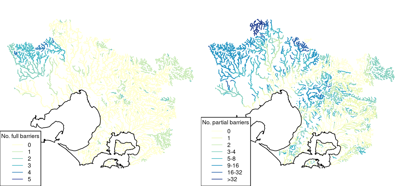
subcs_n_bar$n_part_2023 <- n_bar_2023$n_part_barriers_ds_2023The resulting values for n_full and n_part for the two years were saved as n_full_barriers_ds_1996, n_part_barriers_ds_1996,n_full_barriers_ds_2023 and n_part_barriers_ds_2023 in the subc_env table. The distribution of the numbers of downstream full and partial barriers across the (sampleable) reaches of the network in 2023 is illustrated in Figure 10.2.
The calculation of downstream barriers in 1996 for the full network took > 3 h. The function recalc_barriers()2 permits rapid recalculation of the numbers of downstream for other years. The code used the function to calculate n_full_barriers_ds_2023 and n_part_barriers_ds_2023 in the subc_env table, taking just 23 s. The function takes the 1996 partial and full downstream barrier counts and:
subtracts fishways that had become effective by the given year (
eff_yearargument of the function), using theyear_became_effectivefield of the fishways table, andadds any barriers newly constructed by eff_year, using the
date_constructedfield of the stream_barriers table. Currently, the only confirmeddate_constructedvalues are for the streamflow gauges constructed by the University of Melbourne. Further information on barrier construction dates is lacking.
Because the recalc_barriers() function is rapid, we have included only barrier counts for 1996 and 2023 in the subc_env table, and encourage users to use the function to calculate full and partial barrier counts for other years of interest. The following code illustrates that the number of full downstream barriers in the year 2000 was unchanged from 1996, but had reduced for 57,257 reaches by 2018 (primarily because of the construction of the Dights Falls fishway in the lower Yarra River). The 14 fishways constructed on partial barriers up to the year 2000 reduced the number of downstream partial barriers for 12,386 reaches, and ongoing fishways construction to 2018 reduced downstream partial barriers for 57,257 reaches. These calculations (for the entire stream network) took <20 s for 2018, and <5 s for 2000.
# Assumes a database connection called db_m has been created
subcs <- DBI::dbGetQuery(db_m,  "SELECT site, n_part_barriers_ds_1996,
                                 n_full_barriers_ds_1996 FROM subc_env;")

system.time({
n_bar_2018 <- recalc_barriers(eff_year = 2018, mwstr_connection = db_m)
})  # 17 s for 2018.
# Note that the function returns two values (n_full_barriers_ds_XXXX and
# n_part_barriers_ds_XXX), where XXXX = eff_year.

system.time({
n_bar_2000 <- recalc_barriers(eff_year = 2000,  mwstr_connection = db_m)
})  # 4 s for 2000.

subcs$n_full_barriers_ds_2018 <-
  n_bar_2018$n_full_barriers_ds_2018[match(subcs$site, n_bar_2018$site)]
subcs$n_part_barriers_ds_2018 <-
  n_bar_2018$n_part_barriers_ds_2018[match(subcs$site, n_bar_2018$site)]
subcs$n_full_barriers_ds_2000 <-
  n_bar_2000$n_full_barriers_ds_2000[match(subcs$site, n_bar_2000$site)]
subcs$n_part_barriers_ds_2000 <-
  n_bar_2000$n_part_barriers_ds_2000[match(subcs$site, n_bar_2000$site)]

sum(subcs$n_part_barriers_ds_2018 < subcs$n_part_barriers_ds_1996) # 54245
sum(subcs$n_full_barriers_ds_2018 < subcs$n_full_barriers_ds_1996) # 57257

sum(subcs$n_part_barriers_ds_2000 < subcs$n_part_barriers_ds_1996) # 12386
sum(subcs$n_full_barriers_ds_2000 < subcs$n_full_barriers_ds_1996) # 0
10.4 Calculation of distance and no. barriers between reaches
The calculation of downstream barriers can be expanded to provide detailed information on flow distances between any two reaches in the stream network. The function flow_dist_a_to_b() (in mwstr_network_functions.R) rapidly calculates distances downstream and upstream between two nominated sites, and returns the number of partial and full barriers in each direction. For instance, the flow distance between Watsons Creek at Eltham-Yarra Glen Rd, Watsons Creek downstream to its confluence with the Yarra River and upstream to the Yarra River at Rd 21, above the upper Yarra Reservoir is calculated as:
# Assumes a database connection called db_m has been created (see section 1.2)

flow_dist_a_to_b("WTS_4913", "YAR_13454",
                 mwstr_connection = db_m, year = 2023)
pathway downstream_km upstream_km
1 stream 7.752294 143.89837
2 channel 0.000000 0.00000
3 through large waterbodies 0.000000 9.40712
4 pipe 0.000000 0.00000
5 estuary 0.000000 0.00000
6 marine 0.000000 0.00000
7 no. part barriers 2023 1.000000 4.00000
8 no. full barriers 2023 0.000000 1.00000indicating a 7.8 km flow distance to the confluence with the Yarra over no barriers in 2023 (a fishway having been constructed on Watsons Creek in 2008), and 143.9 km up the river, including 9.4 km through the reservoir, past 3 barriers, including 1 full barrier (the reservoir).
To expand this example, in the code below we quantify distances from the Watsons Creek reach to a) a site downstream, b) the example above of to a site in the same catchment but on a different tributary, c) to a reach in a different stream that also flows into Port Phillip Bay, and d) to a reach in a different stream that flows to a different bay. The result (excluding barrier information) is summarised in Table 10.3. If the two reaches drain to separate outlets, the marine distance is reported schematically as 1 = same marine segment; 2 = different segments, same bay; 3 = Segments separated by Bass Strait; 4 = Murray River to MW region (or other inland terminal).
# Watsons Creek at Eltham-Yarra Glen Rd, Watsons Creek to...
d1 <- flow_dist_a_to_b("WTS_4913", "YAR_275306", mwstr_connection = db_m)
           #  ..Yarra River at Fitzsimons Rd, Templestowe
d2 <- flow_dist_a_to_b("WTS_4913", "YAR_13454", mwstr_connection = db_m)
           # ...Yarra River at Rd 21, Upper Yarra Res Catchment
d3 <- flow_dist_a_to_b("WTS_4913", "KRT_27435", mwstr_connection = db_m)
           # ...Kororoit Ck at Federation Trail, Brooklyn
d4 <- flow_dist_a_to_b("WTS_4913", "BAS_23334", mwstr_connection = db_m)
           # ...Bass River at McGrath Rd, Glen Forbes Sth"
# Extract relevant distances from the four flow_dist_a_to_b calculations.
dist_tab <- cbind(d1, d2[,-1], d3[,-1], d4[,-1])[1:6,]
dist_tab[,-1] <- round(dist_tab[,-1])
names(dist_tab) <- c("Pathway", "D/S ", "U/S ", "D/S ", "U/S ", "D/S", "U/S", "D/S ", "U/S ")
if(knitr::is_html_output()){
ft <- flextable::flextable(dist_tab)
ft <- flextable::autofit(ft)
ft <- flextable::add_header_row(ft,
values = c("","to YAR_275306","to YAR_134454",
"to KRT_27435","to BAS_23334"),
colwidths = c(1,2,2,2,2))
ft
}else{
dist_kab <- knitr::kable(dist_tab)
dist_kab <- kableExtra::add_header_above(dist_kab, c(" " = 1,
"to YAR_275306" = 2,
"to YAR_134454" = 2,
"to KRT_27435" = 2,
"to BAS_23334" = 2))
dist_kab
}to YAR_275306 | to YAR_134454 | to KRT_27435 | to BAS_23334 | |||||
|---|---|---|---|---|---|---|---|---|
Pathway | D/S | U/S | D/S | U/S | D/S | U/S | D/S | U/S |
stream | 33 | 0 | 8 | 144 | 65 | 6 | 65 | 10 |
channel | 0 | 0 | 0 | 0 | 1 | 0 | 1 | 0 |
through large waterbodies | 0 | 0 | 0 | 9 | 0 | 0 | 0 | 0 |
pipe | 0 | 0 | 0 | 0 | 0 | 0 | 0 | 0 |
estuary | 0 | 0 | 0 | 0 | 22 | 2 | 22 | 6 |
marine | 0 | 0 | 0 | 0 | 2 | 3 | ||
The waterbodies database (named
mwb) is stored on the same server as the mwstr database. For further information contact Yung En Chee↩︎the
recalc_barriers()function is in the script mwstr_network_functions.R↩︎