Melbourne Water stream network: user’s manual

6.1 Introduction

This chapter describes the derivation of raster tables of impervious cover (roofs, and asphalt and concrete ground surfaces) and the reach and catchment imperviousness metrics, total and effective imperviousness (TI and EI) derived from the rasters. TI is an important measure of urban density, while EI (in various forms, but generally weighting impervious cover by drainage connectivity to streams) can be considered a measure of urban stormwater impact.

Base data of impervious surface cover for the years 2005, 2014, 2018, and 2022 (from which I derived TI and EI metrics in the cat_env, and subc_env tables) are stored in a 5-m gridcell raster table (r_imp_series, see the stream network download page) with 4 layers: imp_2005, imp_2014, imp_2018 and imp_2022. Note that, in contrast to the case for tree cover (Chapter 7), there is no need to derive a pre-European ‘reference’ table for impervious cover, as it can assumed that the reference state throughout the region is zero impervious cover. The derived metrics, total imperviousness (TI: ti_2005, ti_2014, ti_2018, ti_2022) and effective imperviousness (EI: ei_2005, ei_2014, ei_2018, ei_2022) are stored in the the cat_env table.

6.2 Impervious coverage maps

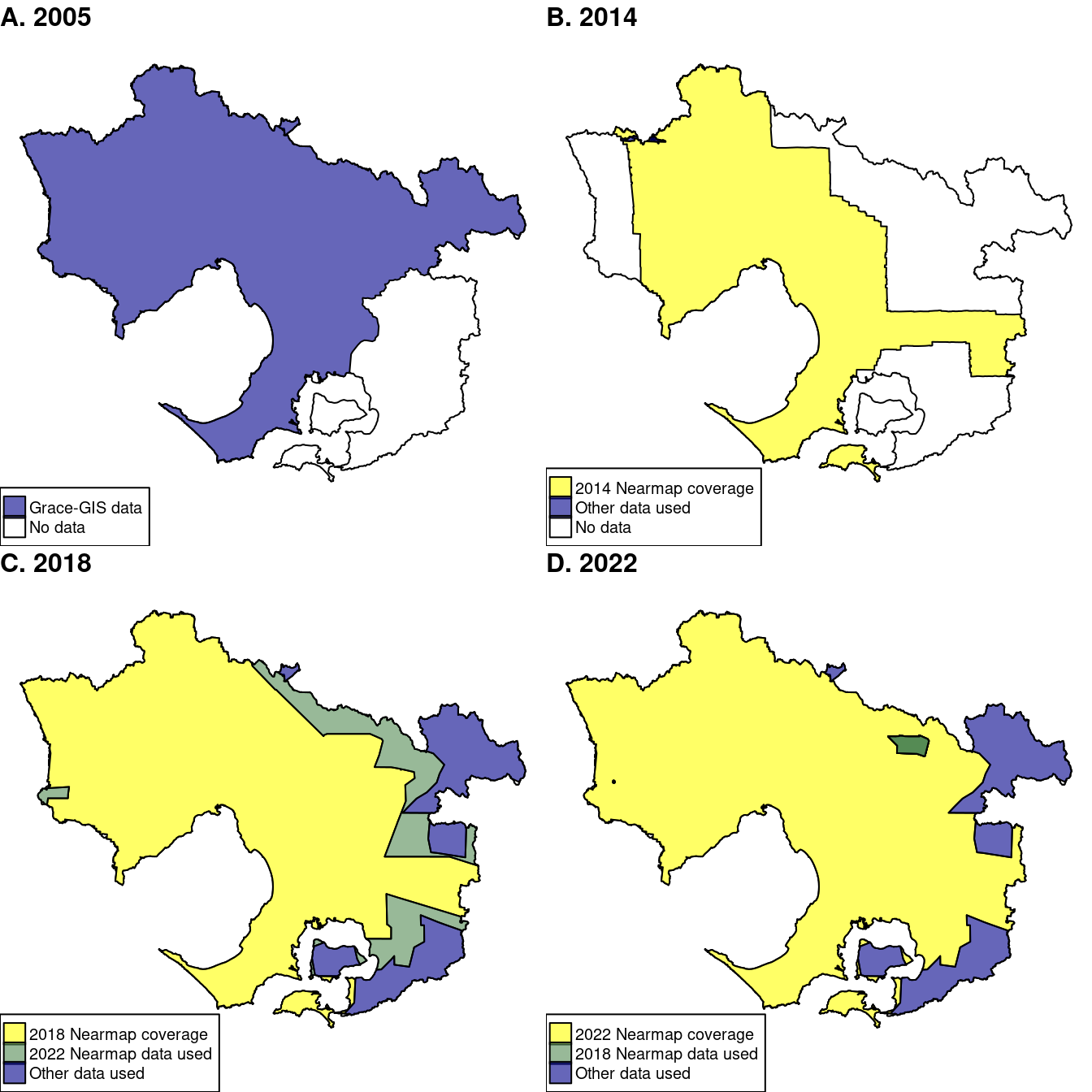
2005 total impervious coverage polygon data was mapped for most of the region (excluding the south-eastern catchments Figure 6.1 A) by automatic classification using a Normalised Differential Vegetation Index (NDVI) from 35-cm resolution, fast-look aerial photos with an infra-red band, followed by a manual verification process (Grace Detailed-GIS Services 2012).

More accurate impervious coverage polygon data were derived for most of the region from Nearmap AI-Pack data for 2014, 2018 and 2022. I defined impervious areas as the combination of Nearmap’s Building footprint, Asphalt, and ConcreteSlab layers. An initial pilot study confirmed that these layers are highly accurate representations. While the building footprints layer explicitly excludes rooftops used by people, such surfaces are covered by ConcreteSlab or Asphalt. Nearmap’s HardSurface layer in their surface permeability pack has the potential to serve as an indicator of impervious surface coverage. In some forested areas that I checked, HardSurfaces more accurately represented the width of sealed roads than the asphalt layer (which marginally underestimated width). However, in other large areas (in the Yarra Ranges), HardSurfaces omitted most impervious surfaces and Asphalt and ConcreteSlab layers were more accurate. I thus chose to use the combination of roofs, asphalt and concrete because of its more consistent accuracy across the region.

The nearmap layers Surfaces_RoadDrivableSurface and Surfaces_Driveway include all roads and driveways regardless of surface, suggesting that the difference between these and impervious surfaces could be used to estimate unsealed road surface coverage. I have not pursued this, but it could be added to the database in the future.

Each dataset had unique gaps in coverage. For the 2018 and 2022 data, I filled the gaps with appropriate data from other sources (Figure 6.1). A larger area was missing data in 2018 than in 2022, although small areas around Warburton (east) and Little River (west) covered by the 2018 data, were missing from the 2022 data. None of these areas saw large changes in urban land or forest cover between 2018 and 2022 (although there may have been some logging coups cleared in the Yarra Ranges). Therefore, land cover estimates for the missing areas were filled by Nearmap data from the nearest year with data where available (green areas in Figure 6.1).

The larger area of missing data from 2014 data included small areas of active urban development between 2014 and 2018. Estimates of 2014 cover per subcatchment were made for those areas, and elsewhere 2018 impervious cover was assumed (see below).

Figure 6.1: Area of available land cover data from various sources in A. 2005, B. 2014, C. 2018 and D. 2022. THe missing areas in each year were estimated from alternative data sources: where Nearmap data was available from the neighbouring year, it was used (green). Otherwise other data sources were used as described in the text.

Areas with no Nearmap data in 2014, 2018 or 2022 (blue areas in Figure 6.1 B-D) were filled with data from several sources. For these rural areas, we created road polygons by creating buffers around 2022 Open Street Map (OSM) lines for roads classed as sealed . All minor roads were assigned a width of 7 m, and large highways 12 m. We used roof polygons estimated from 2009 Lidar as part of an earlier project, and augmented these with hand-drawn polygons of new buildings and paved surfaces visible in 2022 Google satellite imagery.

A small mainly forested area in the northwest of the region was obscured by cloud in the 2014 imagery (Figure 6.1 B): for these areas impervious cover was assumed zero and tree cover (Chapter 7) was filled in those areas from 2018 imagery. For estimates of imperviousness, the 2004 impervious cover raster was not augmented, but estimates were made when compiling subcatchment data (see below).

For all three years, the nearmap data did not cover the full extent of the subcatchment boundaries around the edges of the region. This was an insignificant omission for impervious surfaces, but the missing areas were filled with manually drawn polygons from available imagery for missing vegetation (Chapter 7).

6.3 Catchment total imperviousness estimation

To estimate imperviousness for stream reaches and catchments, I rasterised the polygon data. For all except the 2005 data, I first rasterized the polygons to 1-m gridcells, and then aggregated the 1-m data to 5-m gridcells that match the DEM and flow rasters (see Chapter 3). Each gridcell containing any impervious coverage thus has a value between 1 and 25 representing the impervious area in m². The less accurate 2005 data was rasterised directly to 5-m gridcells, and each gridcell classified as impervious was given a value of 25 to be consistent with the other rasters.

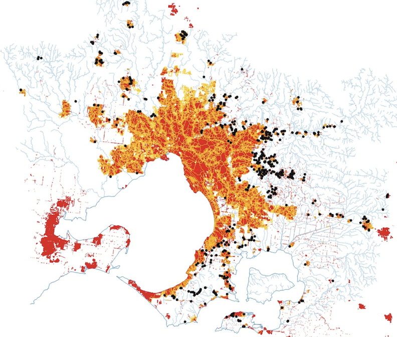
The resulting raster layers are shown in Figure 6.2.

Figure 6.2: Raster data for impervious coverage in A. 2005, B. 2014, C. 2018 and D. 2022. Colors represent the area of impervious surfaces (in m²) in each 25 m² gridcell. For 2005 and 2014, the are covered by available data is indicated by dashed lines.

Comparing growth in total impervious area in the portion of the region (Figure 6.3 B) covered by all four datasets with Melbourne’s population growth (Figure 6.3 A) confirms that growth in impervious surfaces matched population growth well from 2014 to 2022. (Population growth over the 8 years was 19.2%, compared to 22.7% growth in impervious cover).

Figure 6.3 B also shows that the 2005 impervious estimates are not directly comparable to the later Nearmap estimates. The 2005 data tended to overestimate road widths and roof areas, and include gravel surface resulting in perhaps a 15-20% overestimate in coverage. Care should thus be taken using the 2005 data together with the more reliable later data. It can however be useful for identifying developed areas that were undeveloped in 2005.

Figure 6.3: A. Melbourne population size in the 4 years for which impervious data are available (from (https://www.macrotrends.net/cities/206168/melbourne/population) and B. corresponding estimates of total impervious coverage in the portion of the regions covered by all four datasets.

Total impervious area in each subcatchment was calculated from the r_site raster and the four impervious rasters (Figure 6.2) using the following code (showing 2014 data as an example). TI, the area of all impervious surfaces in the upstream catchment as a proportion of total catchment area, was calculated using the approach used to calculate catchment area (Chapter 4). Figure 6.4) shows the resulting patterns of imperviousness in sampleable streams for the four years.

r_imp_2014 <- c(r_imp$imp_2014)
imp_by_site <- terra::zonal(r_imp_2014, r_site, fun=sum, na.rm = TRUE)
names(imp_by_site) <- c("site","sc_tia_2014_m2")
# For 2014 missing impervious data were filled by populating sc_tia_2014_m2
# with 2018 data except for 6 sites in Woori Yallock, and 33 sites in Wallan
# for which 2014 estimates were made from from 2005, 2022 imagery and 
# the difference between 2018 and 2022
subcs <- subcs[order(subcs$nus, subcs$agg_order),]
subcs$sc_tia_2014_m2 <- 
  imp_by_site$sc_tia_2014_m2[match(subcs$site, imp_by_site$site)]
# All subcatchments of agg_order 1 have no subcatchments upstream. 
subcs$tia_2014_m2[subcs$agg_order == 1] <- 
  subcs$sc_tia_2014_m2[subcs$agg_order == 1]
# Loop through remaining subcatchments, adding its imp area to the (already
# calculated) catchment imp areas of subcatchments immediately upstream
for(i in min(which(subcs$agg_order == 2)):nrow(subcs)){
  if(sum(is.na(subcs$carea_m2[subcs$nextds == subcs$site[i]])) > 0) stop("1")
   subcs$tia_2014_m2[i] <-
      sum(subcs$tia_2014_m2[subcs$nextds == subcs$site[i]], 
      subcs$sc_tia_2014_m2[i], na.rm = TRUE)
}
cat_env$tia_2014_m2 <- subcs$tia_2014_m2[match(cat_env$site, subcs$site)]
cat_env$ti_2014 <- cat_env$tia_2014_m2/cat_env$cat_area_m2_r

Figure 6.4: Total catchment imperviousness (TI) as a proportion of total catchment cover for A. 2005, B. 2014, C. 2018, and D. 2022.

6.4 Effective imperviousness estimation

TI assumes all impervious surfaces in an area are of equal importance. However, impervious surfaces of a catchment can differ in their influence on downstream receiving waters. This proposition underlies the concept of effective imperviousness, EI, where ‘effective’ connotes the magnitude of each impervious surface’s effect on a receiving water. EI thus weights each impervious according to its inferred effect. Imperviousness (I) in general is calculated as:

\[ I = \frac{\Sigma^n_1{IA}_i \cdot W_i}{CA} \tag{6.1}\]

where \({IA}_i\) is the area of the ith of n impervious surfaces in a catchment of area CA, each weighted by \(W_i\). For TI, \(W\) = 1 for all surfaces. For EI, \(W_i\) is usually a proportional weighting related to the degree of drainage connection between the surface and the receiving water (Walsh, Burns, Fletcher, et al. 2022). Conventional stormwater drainage (Burns et al. 2012) creates a hydraulically efficient connection between impervious surfaces and the pipe outlet, and the simplest formulation of EI is to give surfaces draining directly to a sealed stormwater drain or pipe a weighting of 1 and surfaces that drain informally to pervious surfaces a weighting of 0 (Walsh, Burns, Fletcher, et al. 2022).

Such a weighting scheme does not adequately model degrees of connection that might arise from:

different distances of overland flow for informal drainage, or from upslope outlets of stormwater drains;
differences in hydraulic efficiency of pervious surfaces along the flow path to the stream; or
interception by stormwater control measures (SCMs).

I have adopted a measure of EI that accounts for the first of these effects (overland flow distance). There is insufficent soil and vegetation data available¹ to permit a region-wide estimate of the second effect (hydrualic efficiency). For version 1.3 of the stream network, a region-wide database of SCM location and performance (to account for the third effect) was unavailable. However, I demonstrate below how the effects of SCMs could be calculated below for a small area for which SCM data is available (after Walsh, Burns, Fletcher, et al. 2022).

Walsh and Kunapo (2009) calculated an EI variant, which they termed attenuated imperviousness (AI), by weighting all impervious surfaces by the overland flow distance of their most downstream edge to the nearest stormwater drain or stream (whichever was reached first). They found the optimal weighting for the prediction of a macroinvertebrate assemblage metric to be:

\[ W = e^{-dL/13.56133} \tag{6.2}\]

where W is the weight as in Equation 6.1, and dL is the overland flow distance to drain or stream in m. A logical problem with that approach was that the weighting conflates the attenuating effect of overland flow distance on impervious runoff with the decreasing probability that an impervious surface is connected to the stormwater pipe the further it is from the pipe.

The full impact of directly drained (i.e. connected) impervious surfaces is transmitted to the stream at the end of the pipe. Thus directly connected impervious surfaces should be unweighted: effectively a flow distance of zero, and distance-related attenuation should only be applied to informally drained impervious surfaces. To allow such a weighting scheme, I used the council stormwater drainage network maps, and aerial and street-view imagery, to estimate a) which areas of urban development are likely to be connected to the stormwater drainage system, and b) the location of stormwater drainage outlets where they drained to the hillslope rather than directly to the stream.

Ground-truthing (e.g. Figure 6.5) suggests that >~95% of impervious surfaces in developed residential and commercial areas that are serviced by council stormwater drainage pipes drain directly to those pipes (not accounting for formal SCMs such as rainwater tanks or rain-gardens, considered below). Thus, applying a weighting of 1 to impervious surfaces in all such areas and a distance-related weighting to all other impervious surfaces avoids the conflation problem of AI described above.

Figure 6.5: An example of connection classification of impervious surfaces from a well-studied catchment (Walsh, Burns, Fletcher, et al. 2022). The blue line in the north indicates the receiving stream, and the network of orange lines indicates council drainage pipes. Ground truthing allowed accurate identification of the roof and paving surfaces that drain directly to the council drainage pipes (or to the stream in the case of the house to the north of the road) (black polygons). The road running east-west is informally drained to a swale. It and a small proportion of driveways and small buildings were informally drained to gardens, and are considered unconnected (grey polygons). The yellow open polygons are from the *conn_subcs* table drawn to capture all impervious surfaces connected to drainage pipes.

I compiled the table conn_subcs, which maps all areas serviced by council stormwater pipes and the table conn_pps, which identifies any upslope stormwater pipe outlets (Figure 6.6).

Figure 6.6: Connected impervious catchment polygons of the *conn_subcs* table (orange) and outlet points for those catchments with upslope outlets (black), overlaying the sampleable stream network (blue) and the stormwater drainage network (red). Some stormwater pipes are not within a catchment polygon because a) stormwater network extends beyond the stream network region and b) there are many small segments of stormwater pipe mapped that are culverts under roads that do not concentrate impervious runoff sufficiently to warrant adjusting flow distance for those impervious surfaces.

The conn_subcs and conn_pps tables were compiled as follows. I first selected all subcatchments within the 2002 urban growth boundary (UGB) as primary candidates that are likely to be near-fully connected and saved this as the working version of conn_subcs. Several steps of manual correction were then made in QGIS.

Stormwater drainage pipes outside the UGB were inspected, and subcatchments fully serviced by stormwater pipes were added to the fully connected subcatchment layer. Each subcatchment was inspected with base layers of imagery and stormwater drainage pipes. In some areas, the stormwater drainage network extended beyond the topographic subcatchment boundary. Some conn_subc polygons thus extend beyond the boundary of the subcatchment with the equivalent site code in the subcs table.
Areas of catchments that do not drain to the stormwater pipes were clipped from the conn_subcs subcatchment. Roads without curbs draining to swales (confirmed using Google Streetview) were considered to be not draining to pipes. In some peri-urban developments, swales sat above stormwater pipes. In such cases, unless there was evidence otherwise, the buildings along the streets were assumed to drain to the stormwater pipes, while the roads were considered unconnected.
Any pipe outlets distant from the stream were added to the conn_pps table, given a unique id, in addition to the site code of the subcatchment, which was recorded. In some cases (e.g. pour point fid=1), a single pourpoint was added for several adjacent outlets in the same subcatchment that drain to the same drainage line (where the flow distances to the stream are of a similar magnitude). Where a pipe flows into a terminal stormwater control measure (SCM) such as a wetland, the pourpoint was placed at the outlet of the SCM, (to allow the effects of SCMs to be modelled separately: see below).
Subcatchments in the UGB were reviewed systematically, searching for any areas without stormwater drainage and for any pipe outlets upslope of stream lines. In such cases the subcatchment boundaries were amended and pourpoints added as required. Some new development areas visible on aerial imagery did not have mapped stormwater drainage, but were inferred to drain to stormwater drainage from their development density and curbed roads.

EI was then calculated for the region as follows.

Distance to stream (field d2str_m) was extracted from the r_d2str raster for every point in the conn_pps table using the terra::extract() command.
Distance to stream (field d2str_m) was set to zero for all polygons table conn_subcs, except for those with a matching point (by fid in conn_pps and pp_fid in conn_subcs), for which d2str_m = the distance-to-stream value of the pipe outlet from conn_pps.
New rasters depicting distance-to-stream, effective-impervious-area (EIA), and site were calculated using the conn_subcs table to adjust the r_d2str and r_site rasters to account for flow distance and subcatchment boundary changes made by the stormwater drainage network (see the following code). The weighting used to calculate EIA was the optimal weighting determined by Walsh and Kunapo (2009) (Equation 6.2) The optimality of this weighting should be reviewed given the different approach to assessing connection and the superior new impervious coverage data.

r_site <- terra::rast(paste0(mwstr_dir,"/r_site.tif"))
# use r_site as a template to rasterize conn_subcs
r_d2str_conn <- terra::rasterize(conn_subcs, r_site, field = "d2str")
# replace d2str values for conn_subcs areas 
r_d2str_conn <- terra::cover(r_d2str_conn, r_d2str)

# calculate and EIA raster using the optimal Walsh Kunapo weighting
r_conn_eia <- r_imp * exp(-r_d2str_conn/13.56133)

# create a new site raster, allowing for boundary adjustments in conn_subcs
r_conn_site <- terra::rasterize(conn_subcs, r_site, field = "site")
r_conn_site <- terra::cover(r_conn_site, r_site)

# calculate EIA for each subc, setting NAs to zero where there was no imp area
eia_by_site <- terra::zonal(r_conn_eia, r_conn_site, fun=sum, na.rm = TRUE)
for(i in 2:ncol(eia_by_site)){
  eia_by_site[is.na(eia_by_site[,i]),i] <- 0
}

Catchment EI was then calculated by aggregating all upstream EIA and dividing by catchment area using code similar to that used to calculate TI above.

The following illustrates the above EI calculation graphically for Wattle Valley Creek, in the Little Stringybark Creek catchment. Estimates of stormwater control measure performance are available for this catchment, permitting an extension of EI estimation to account for stormwater control (EI_s). Such a calculation is currently not possible for the whole network, but will be if an adequate database of SCM specifications for the region is assembled. Figure 6.7 A shows the Wattle Valley Creek catchment boundary over 2022 nearmap imagery. Figure 6.7 B overlays the nearmap AI-pack roof (ochre) and concrete/asphalt surfaces (grey), and Figure 6.7 C overlays the stormwater drainage network (red). Figure 6.7 D shows the locations of pipe outlets and the subcatchment boundaries of those pipe networks (determined in this example by Walsh, Burns, Hehir, et al. (2022), and stored in the conn_subcs table).

Figure 6.7: Wattle Creek, Mt Evelyn, with 2022 Nearmap imagery A. catchment boundary, B. with Nearmap polygon data of concrete and asphalt (grey) and roofs (ochre), C. with council stormwater pipes added, and D. with stormwater pipe catchments (enclosing all impervious surfaces inferred to be draining to each pipe) and their points of discharge.

Figure 6.8 A shows the 5-m gridcell distance-to-stream raster r_d2str (see Chapter 3) cropped to the catchment boundary. Figure 6.8 C is the distance-to-stream raster adjusted so that the distance to stream for each pipe subcatchment equals the distance from the pipe outlet to the stream (zero in all but one cases in this example). To calculate EI, the gridcell values of the impervious raster (derived from the nearmap polygons as described above to give a value between 1 and 25 approximating the area of impervious coverage in each 25-m² gridcell). The resulted weighted areas are illustrated in Figure 6.8 C.

The Wattle Creek catchment was chosen as an example, as it contains many SCMs installed as part of the Little Stringybark Creek catchment, allowing an estimation of the integrated performance at the outlet of each pipe: the stormwater control index, S, developed by Walsh, Burns, Hehir, et al. (2022). For the seven pipe catchments in this example catchment, S ranged from 0.14 (for the pipe catchment in which large stormwater harvesting projects were possible) to 0.47. Figure 6.8 D shows the weighted areas multiplied by S. To calculate TI, the summed area of impervious surfaces was divided by the catchment area (10.1%). EI not accounting for SCMs used the weighted sum or impervious areas as in Equation 6.2 (Figure 6.8 C, 5.3%). For EI_s (accounting for SCMs) W was multiplied by S (Figure 6.8 C, 1.5%).

Figure 6.8: Wattle Creek, Mt Evelyn, with a total Imperviousness (TI) of 10.1% illustrating calculation of effective imperviousness assuming no effect of stormwater control measures (EI) and EI_s, accounting for SCM performance. A. Flow distance to stream without adjusting for connection to stormwater drainage (using the stormwater pipe catchments shown in Figure 6.7 D). B. Flow distance to stream with areas flowing to stormwater pipes given the flow distance from the pipe outlet to the stream (0 in most cases). C. Weighted impervious area (IA) applied to impervious areas (IA * exp(-dL/13.56133), where dL is the adjusted flow distance as in B, used to calculate EI. D. Weighted impervious area as in C, but additionally multiplied by S, the fractional measure of SCM performance, used to calculate EI_s. For C and D, the weighted values range between 0 and 25: the area of impervious surface in each 25 m₂ gridcell.

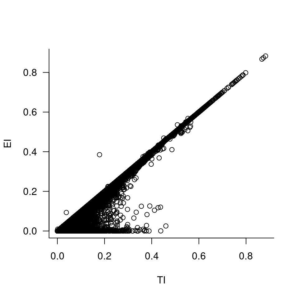
TI and EI across the region are strongly correlated (Figure 6.9), but importantly there are many catchments with TI between 2 and 40% that have very low EI, providing potential for robust tests of different variants of imperviousness as predictors of stream response. While EI is less than or equal to TI in almost all reaches, this is not the case for a small number (Figure 6.9) as result of stormwater pipes extending beyond catchment boundaries.

Figure 6.9: The relationship between total imperviousness (TI) and effective imperviousness (EI) for all reaches in the stream network in 2018 (as an example: a similar relationship for other years).