Appendix A — Stream and subcatchment assembly methods
Joshphar Kunapo and Christopher J Walsh
Compilation of the stream lines and subcatchments was primarily done by Joshphar Kunapo (initially of Grace Detailed-GIS Services and later of the University of Melbourne), in collaboration with CJW
A.1 Streams
We chose to build the new stream network by adopting, adjusting and augmenting where necessary, the lines in the DR_Natural_Waterway_Centreline to retain links to the MI_PRINX asset identifications in the original data. We developed flow lines using an unconditioned LiDAR DEM with ESRI ArcHydro tools. We used these flow lines, in conjunction with a hillshade model (from the LiDAR DEM) to adjust the alignment of DR_Natural_Waterway_Centreline, DR_Channel_Centreline and DR_Waterways_above_MW_Limit lines.
The Melbourne Water layers DR_Channel_Centreline and DR_UGround_Centreline were added to the stream lines where necessary to ensure a continuous hydrologically connected network. The complete DR_UGround_Centreline layer was not used, but we have retained all pipes that connect upland sections of streams with either their outlet to the sea or with more downstream sections of streams or channels. We have also retained small segments of pipes at their outlets to the sea or to streams. There were instances where the direction of the lines in the Melbourne Water layers were upstream. These were adjusted manually. Thus a non-duplicated, non-overlapping, fully node-to-node connected network was developed.
Version 1.1 was the product of several iterations as part of several projects, led by Grace Detailed-GIS Services, using data from different LiDAR acquisitions, and has resulted in results of varying quality across the region.
The first project added upstream extensions to the DR_Natural_Waterway_Centreline layer, using 2009 LiDAR data where available (Fig A1-1A), and a lower-resolution DEM derived from available contour maps (5–10-m intervals) for the rest of the region. Lines with type = stream extensions
in the area covered by the 2009 LiDAR are therefore of high quality.
The second project, was commissioned in 2019 to correct alignments of lines from the first project with stream order > 2 in areas covered by the 2018 LiDAR acquisition. Alignments of stream lines with stream order >2 are therefore of high quality in the area covered by the 2018 LiDAR.
The third project was commissioned in 2020 after Melbourne Water discovered that we had compiled the stream network without reference to the DR_Waterways_above_MW_Limit layer, of which we were unaware. (For this project we also discovered the existence of the 2016 LiDAR data, which we were unaware of when conducting the second project; Fig. A1-1B.) This project required checking of the DR_Waterways_above_MW_Limit layer and correcting the alignment and adding any of the lines in that layer that were omitted from previous versions (including adding nodes and splitting the existing lines to ensure hydrologic connectivity of the network). This step was taken in collaboration with Melbourne Water staff, and it was agreed that small cut drains without a clear place in the dendritic hydrologic network would not be included in the final product. The added lines in areas (including in areas outside the 2009 LiDAR extent) are of high quality.
The process of the third project involved substantial manual checking, correction and augmentation across the network, particularly in areas such as the southern slopes of Mt Donna Buang, where we had ground-truthed data on headwater locations. This process of manual checking identified that further re-alignment and augmentation of headwater streams in the areas outside the 2009 LiDAR area (Fig. A1-1A), and further re-alignment of some larger streams in the upper Yarra (greyscale area in Fig. A1-1B) are still required. While alignments are broadly of high quality in these areas, Fig. A1-2 show examples of two areas in the upper Yarra region with larger streams needing re-aligment, and some small tributary channels requiring addition.
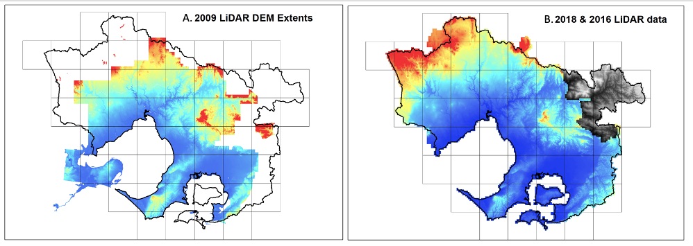 Fig. A1-1. The Melbourne Water region (black-bordered polygon) and LiDAR availability in three years. A. Extent of LiDAR acquisition in 2009 (spectral colouring); B. Extent of LiDAR acquisition in 2018 (spectral colouring) and in 2016 (grey-scale).
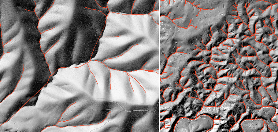 Fig. A1-2. Screenshots of the hillshade model in two parts of the Upper Yarra catchment, with the stream layer in red, to illustrate areas of low-quality alignment and some missing headwater streams from the final product (left panel), and an area where the stream delineation is of high quaity (right panel) for comparison.
Version 1.2 revised and corrected line delineation and extent in areas with errors such as those illustrated in Fig. A1-2 using hillshade derived from the 2016-2018 LiDAR, which covered the entire region (except for a very small portion of the upper Yarra catchment).
A.2 Subcatchments
We developed the subcatchment layer by:
- producing an engineered 5-m cell-size Digital Elevation Model (DEM) by forcing the stream network lines and council pipes into the original LiDAR DEM. Any sinks were identified and removed to develop the final hydrological DEM1.
generating flow direction and flow accumulation grids, using the ArcGIS hydrological tools, and then deriving a 1-ha drainage network from flow accumulation model to ensure a minimum subcatchment area of 1 ha.
identifying the pour points to which the subcatchments should be derived on a 1-ha drainage network.
At the most upstream point of each stream. Because the line vectors did not necessarily sit on the optimal cell of the flow accumulation grid, these points were snapped to the nearest optimal flow accumulation cell of 5m raster.
At council pipe-stream confluences of the stream network. This was laborious because most of the council-pipe lines are not digitized to touch streams at their confluence. Because it was difficult to manually fix these gap for the entire region, the engineered DEM was used to create an automated network at a scale that represents the council pipe network and its relation to the stream network. Pour points upstream of confluence were selected from this automated network.
At stream-stream confluences of the stream network. These confluence points were first identified from the original stream network. Then the pour points from the automated network within a threshold of the original were identified. Further upstream-downstream tracing methods were used to identify the best confluence points to represent the original vector-based confluence points.
Between confluences of the stream network to avoid reaches exceeding 500 m long. These points were snapped to the optimal nearest flow cell. Any of these points which were within 100m of existing points generated in steps a-c were ignored.
At the upper limit of estuaries (as currently estimated). These points were also snapped to the optimal nearest flow cell
- With the pour-points selected, subcatchments were developed using ESRI ArcHydro tools. The tool use input pour-points, rasterized stream network and the flow direction grid that was developed from the engineered DEM to derive subcatchments. From this automated subcatchments output, ingle pixel polygons were eliminated, island polygons were fixed and the upstream downstream connectivity for the derived subcatchments were established via next downstream id attribute.
The DEM (
DEM_5m_2018_2016/fill_l5mdem18_16.tif
) and rasters derived from it are most easily accessed from the unimelb directorywergSpatial/MWRegion/Rasters/mwstr_v1.2
. See README in that directory.↩︎