#|

library(terra)

# AWRA source data
url <- paste0("https://dapds00.nci.org.au/thredds/fileServer/iu04/",
              "australian-water-outlook/historical/v1/AWRALv7/")
# downloaded to:
dl_dir <- "/download_directory_of_choice"
# Loop through all years
# for(i in 1911:2022) {
# file_name_web <- paste(url, "qtot_", i, ".nc", sep = "")
# file_name_network <- paste(dl_dir, "qtot_", i, ".nc", sep = "")
# download.file(url = file_name_web, dest = file_name_network)
#   }
#list of the *.nc files
daily_grids <- list.files(dl_dir, pattern = "\\.nc$")
daily_grid_years <- as.numeric(substr(daily_grids,nchar(daily_grids)-6,
                                      nchar(daily_grids)-3))

# Clip to MW region and create a stack of mean monthly runoff rasters.
subcs <- sf::st_read(db_m, query = "SELECT site, nextds, scarea, carea_km2, agg_order, nus, geom FROM subcs;")
subcs_4326 <- sf::st_transform(subcs, 4326)
mw_region <- sf::st_read(db_m, "region_boundary")
# put buffer around region to ensure complete coverage with all 5-km pixels
mw_region <- sf::st_buffer(mw_region,5000)
mw_region_4326 <- sf::st_transform(mw_region, 4326)
mw_ext <- terra::ext(mw_region_4326)

  for(i in 1:length(daily_grid_years)){
    xi <- suppressWarnings(terra::rast(paste0(dl_dir,"/",daily_grids[i])))
    xi <- suppressWarnings(terra::crop(xi,mw_ext))
    if(i == 1){
      mw_annual_grid <- sum(xi, na.rm = TRUE)
    }else{
      mw_annual_grid <- c(mw_annual_grid,sum(xi, na.rm = TRUE))
    }
  }  # 110 s

# Better to reproject the vector subc layer than the raster
subcs_4326 <- terra::vect(subcs_4326)   #17 s

# create Mean annual runoff grids (for various periods)
# 1911-2009 - to match earlier versions of the stream network
mw_meanQ_grid_to_2009 <- terra::mean(mw_annual_grid[[1:98]], na.rm = TRUE)
# 1911-2022 - full record
mw_meanQ_grid <- terra::mean(mw_annual_grid, na.rm = TRUE)

# and extract by subcatchment
system.time({
meanQ_by_subc <- terra::extract(mw_meanQ_grid, subcs_4326, weights = TRUE,
                    fun = mean, na.rm = TRUE, exact = TRUE)
meanQ_to_2009_by_subc <- terra::extract(mw_meanQ_grid_to_2009, subcs_4326, weights = TRUE,
                    fun = mean, na.rm = TRUE, exact = TRUE)
}) # ~ 10 min

meanQ_by_subc$scarea <- subcs$scarea
meanQ_by_subc$meanQ_ML <- meanQ_by_subc$mean * meanQ_by_subc$scarea * 1e-6
meanQ_by_subc$meanQ_ML_to_2009 <- meanQ_to_2009_by_subc$mean * meanQ_by_subc$scarea * 1e-6
meanQ_by_subc <- cbind(meanQ_by_subc, subcs[,c("site","nextds","agg_order","nus","carea_km2")])
meanQ_by_subc <- meanQ_by_subc[names(meanQ_by_subc) != "geom"]
meanQ_by_subc <- meanQ_by_subc[order(meanQ_by_subc$nus, meanQ_by_subc$agg_order),]
meanQ_by_subc$cat_meanQ_ML[meanQ_by_subc$agg_order == 1] <-
  meanQ_by_subc$meanQ_ML[meanQ_by_subc$agg_order == 1]
meanQ_by_subc$cat_meanQ_ML_to_2009[meanQ_by_subc$agg_order == 1] <-
  meanQ_by_subc$meanQ_ML_to_2009[meanQ_by_subc$agg_order == 1]
for(i in min(which(meanQ_by_subc$agg_order == 2)):nrow(meanQ_by_subc)){
    meanQ_by_subc$cat_meanQ_ML[i] <-
    sum(meanQ_by_subc$cat_meanQ_ML[meanQ_by_subc$nextds == meanQ_by_subc$site[i]],
        meanQ_by_subc$meanQ_ML[i], na.rm = TRUE)
    meanQ_by_subc$cat_meanQ_ML_to_2009[i] <-
    sum(meanQ_by_subc$cat_meanQ_ML_to_2009[meanQ_by_subc$nextds == meanQ_by_subc$site[i]],
        meanQ_by_subc$meanQ_ML_to_2009[i], na.rm = TRUE)
}
meanQ_by_subc$cat_meanQ <- meanQ_by_subc$cat_meanQ_ML/meanQ_by_subc$carea_km2
meanQ_by_subc$cat_meanQ_to_2009 <- meanQ_by_subc$cat_meanQ_ML_to_2009/meanQ_by_subc$carea_km28 Flow estimation
Christopher J Walsh and Matthew J Burns
We compiled modelled pre-urban hydrologic data for each reach of the network from the Australian Landscape Water Balance (AWRA-L) model data (Frost and Shokri 2021). The model simulates rainfall-runoff behavior through small unimpaired landscapes (i.e. those free from human impact such as urbanization and water abstraction, but assumes contemporary forest cover). The output we used to estimate streamflow was qtot: the sum of surface runoff, interflow, and baseflow.
The source data was daily gridded runoff data for all of Australia (5-km resolution). We downloaded all available data from 1911 from the (national computational infrastructure site)[https://dapds00.nci.org.au/thredds/catalog.html], and calculated the mean discharge depth for each gridcell for the full record (1911-2022), and for 1911-2009 for equivalence with the measure of mean discharge used in earlier studies of the region (the two values were nearly identical). Spatially weighted means of the mean gridcell values were calculated for all subcatchments, and converted from mm to ML, which we used to sum all upstream discharge for each subcatchment, before dividing by total catchment area to calculated mean catchment discharge as meanq_mm (for the full record) and meanq_mm_to_2009, both stored in the cat_env table.
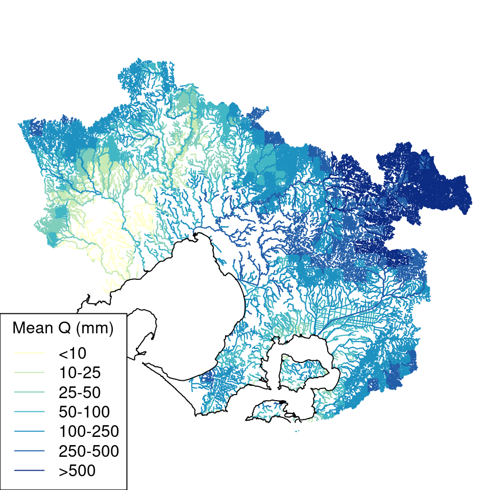
The 5-km gridcells of the AWRA-L data resulted in some tiling of discharge estimates for headwater streams with small catchments (Figure 8.1), but the accumulation of estimates across the catchments of larger streams smoothed these small-scale anomalies (Figure 8.2). The estimates of discharge for small streams should therefore be used with caution
