
7 Tree canopy cover
7.1 Introduction
This chapter describes the derivation of raster tables of tree canopy cover (defined as tree canopies >2 m tall) for the years 1750, 2006, 2018 and 2022, and the reach and catchment forest-cover metrics derived from them. The raster data are stored in the database as a 5-m gridcell raster (r_tree_series.tif) with 4 layers named trees_1750, trees_2006, trees_2018 and trees_2022, and the derived metrics, total forest cover (TF: tf_1750, tf_2006, tf_2018, tf_2022) and attenutated forest cover (AF: af_1750, af_2006, af_2018, af_2022) are stored in the the cat_env table.
Accurate comparable estimates of tree canopy cover in the region over time are a primary management need to track both the loss of tree cover (through many human activities) and the restoration of tree cover (primarily through land and stream management actions). Contemporary tree-canopy cover estimates (polygon data of trees > 2 m tall) were available from two primary sources:
data derived from LIDaR imagery (primarily 2009) along streams and using coarser land use data for land > 200 m from stream lines by Grace Digital-GIS Services for Melbourne Water. These data were manually corrected by the consultants using 2006 imagery (and further corrected for an estimate of 2005 tree cover: see below).
2018 and 2022 Medium & High Vegetation (>2m) from Nearmap’s Vegetation AI pack. The 2014 tree-cover data was not included in analyses given the large area of missing data.
While contemporary tree cover is a good predictor of in-stream state, comparison of contemporary in-stream state with what it might have been in its natural state requires an estimate of tree canopy cover before the arrival of Europeans in the region. I thus derived a reference
dataset for tree canopy cover (total catchment and attenuated forest cover), using the modelled 1750 ecological vegetation class (EVC) spatial data (Department of Environment, Land, Water & Planning 2022) as the representation of pre-European vegetation cover.
7.2 1750 tree canopy cover estimated from EVCs
There are 131 EVCs in the subset of the Victorian EVC 1750 data clipped to the Melbourne Water region, with descriptive names that correspond broadly to structural vegetation classes defined by (Specht 1970): see Table 7.1.
| Life form and height of tallest stratum | Dense (70-100% | Mid_dense (30-70%) | Sparse (10-30%) | Very sparse (<10%) |
|---|---|---|---|---|
| Trees >30 m | Tall closed forest | Tall open forest | Tall woodland | Tall open woodland |
| Trees 10-30 m | Closed forest | Open forest | Woodland | Open woodland |
| Trees 5-10 m | Low closed forest | Low open forest | Low woodland | Low open woodland |
| Shrubs 2-8 m | Closed scrub | Open scrub | Tall shrubland | Tall open shrubland |
| Shrubs <2 m | Closed heath | Open heath | Low shrubland | Low open shrubland |
The structural classification of Specht (1970) does not specify cover ranges for understorey strata, and the EVC classification does not consistently use closed
and open
classifications. Therefore some judgement was required to estimate cover that is consistent with recent estimates of canopy cover of trees >2 m height.
Understorey cover in (1750) forests and woodlands was likely to exceed 2 m height. I assumed that classes described as forest
without descriptors of lower strata, or with descriptors such as shrubby
that are likely to indicate understory canopy > 2 m high, had 100% canopy cover (of strata at least 2 m high). Thus the classes Damp Forest, Lowland Forest, Warm Temperate Rainforest, Riparian Forest, Heathy Dry Forest, Shrubby Dry Forest, Shrubby Foothill Forest, Wet Forest, Box Ironbark Forest, Valley Heathy Forest, Valley Slopes Dry Forest, Herb-rich Foothill Forest/Shrubby Foothill Forest Complex, Montane Damp Forest, Sand Forest, Riparian Forest/Swampy Riparian Woodland Mosaic, Riparian Forest/Swampy Riparian Woodland/Riparian Shrubland/Riverine Escarpment Scrub Mosaic, Cool Temperate Rainforest, Montane Wet Forest, Riparian Forest/Warm Temperate Rainforest Mosaic were assigned cover of 100%.
I added six classes that did not include the term forest into the 100% cover forest class: Swampy Riparian Complex, Riparian Thicket, Lignum Swamp, Montane Riparian Thicket, Red Gum Swamp, No EVC assigned - need editing. The last class consisted of polygon slivers that appeared to be compilation errors and lay among forest polygons.
Using a similar logic, the woodland classes Riparian Scrub/Swampy Riparian Woodland Complex, Gully Woodland, Coast Banksia Woodland/Coastal Dune Scrub Mosaic, Floodplain Riparian Woodland, Granitic Hills Woodland, Riparian Woodland, Swampy Riparian Woodland/Swamp Scrub Mosaic, Coast Banksia Woodland, Montane Dry Woodland, Coastal Headland Scrub/Coast Banksia Woodland Mosaic, Riparian Woodland/Stream-bank Shrubland Mosaic, Sub-alpine Woodland, Shrubby Woodland, Banksia Woodland, Coast Banksia Woodland/Swamp Scrub Mosaic, Plains Swampy Woodland, Grassy Woodland/Swamp Scrub Mosaic were assigned cover of 100%.
Forest classes that indicate low understorey strata without further information about density (Herb-rich Foothill Forest, Valley Grassy Forest, Grassy Forest, Grassy Riverine Forest, Valley Grassy Forest/Herb-rich Foothill Forest Complex, Damp Heathy Woodland/Lowland Forest Mosaic, Swamp Scrub/Plains Grassy Forest Mosaic) were assigned cover of 70%, (at the boundary of Specht’sclosed and open classes). Grassy Dry Forest, and Riparian Forest/Creekline Grassy Woodland Mosaic suggested a more open structure and were assigned cover of 50% (the mean of Specht’s open class).
Woodland classes that indicate low understorey (Plains Grassy Woodland, Heathy Woodland, Swampy Riparian Woodland, Damp Sands Herb-rich Woodland, Grassy Woodland, Swampy Woodland, Damp Heathy Woodland, Damp Sands Herb-rich Woodland/Swamp Scrub Mosaic, Creekline Herb-rich Woodland, Plains Woodland/Plains Grassland Mosaic, Montane Grassy Woodland/Rocky Outcrop Shrubland/Rocky Outcrop Herbland Mosaic, Sedgy Riparian Woodland, Creekline Grassy Woodland, Rocky Chenopod Woodland, Damp Sands Herb-rich Woodland/Heathy Woodland Mosaic, Heathy Woodland/Sand Heathland Mosaic, Sedgy Swamp Woodland, Grassy Woodland/Damp Sands Herb-rich Woodland Mosaic, Plains Grassy Woodland/Swamp Scrub/Plains Grassy Wetland Mosaic, Hills Herb-rich Woodland, Montane Grassy Woodland, Alluvial Terraces Herb-rich Woodland, Damp Sands Herb-rich Woodland/Heathy Woodland Complex, Scoria Cone Woodland, Alluvial Terraces Herb-rich Woodland/Creekline Grassy Woodland Mosaic, Plains Grassland/Plains Grassy Woodland Mosaic) were assigned cover of 30% (the top of Specht’s woodland range).
Scrub
classes (defined by Specht as 2-8 m in height) that were not combined with low classes (Swamp Scrub, Riparian Scrub, Estuarine Wetland/Estuarine Swamp Scrub Mosaic, Swamp Scrub/Wet Heathland Mosaic, Coastal Dune Scrub, Coastal Alkaline Scrub, Coastal Headland Scrub, Blackthorn Scrub) were assigned cover of 100%, and those combined with low strata (Coastal Headland Scrub/Coastal Tussock Grassland Mosaic, Coastal Saltmarsh/Coastal Dune Grassland/Coastal Dune Scrub/Coastal Headland Scrub Mosaic, Coastal Dune Scrub/Coastal Dune Grassland Mosaic, Clay Heathland/Wet Heathland/Riparian Scrub Mosaic, Aquatic Herbland/Swamp Scrub Mosaic, Coastal Dune Scrub/Bird Colony Succulent Herbland Mosaic, Brackish Grassland/Swamp Scrub Mosaic, Coastal Alkaline Scrub/Bird Colony Succulent Herbland Mosaic) were assigned 50% cover.
Shrub
classes (Coastal Saltmarsh/Mangrove Shrubland Mosaic, Berm Grassy Shrubland, Mangrove Shrubland, Stream Bank Shrubland, Escarpment Shrubland, Mangrove Shrubland/Coastal Saltmarsh/Berm Grassy Shrubland/Estuarine Flats Grassland Mosaic, Mangrove Shrubland/Estuarine Flats Grassland Mosaic, Bird Colony Shrubland, Sub-alpine Shrubland) were assigned 30% cover (the top of the range for Specht’s tall shrubland class).
The above classifications left 29 low-vegetation classes and 5 waterbody classes which were assigned 0% cover. The waterbody classes were Water - Ocean, Floodplain Wetland Aggregate, Brackish Lake Aggregate, Water body - salt, Water Body - Fresh. The low vegetation classes Sand Heathland, Wet Heathland, Coastal Saltmarsh, Plains Grassland, Plains Grassy Wetland, Plains Sedgy Wetland, Creekline Tussock Grassland, Brackish Wetland, Bare Rock/Ground, Wetland Formation, Coastal Tussock Grassland, Grey Clay Drainage-line Aggregate, Brackish Grassland, Cane Grass Wetland, Sedge Wetland, Aquatic Herbland, Shallow Freshwater Marsh, Damp Heathland, Reed Swamp, Estuarine Flats Grassland, Clay Heathland, Sub-alpine Treeless Vegetation, Wet Verge Sedgeland, Bird Colony Succulent Herbland, Bird Colony Succulent Herbland/Coastal Tussock Grassland Mosaic, Sand Heathland/Wet Heathland Mosaic, Coastal Dune Grassland, Sub-alpine Wet Heathland/Alpine Valley Peatland Mosaic, Alpine Grassy Heathland.
The spatial distribution of EVC classes grouped into Specht’s vegetation types is illustrated in Figure 7.1, and the spatial distribution of canopy cover following the above reclassifications is illustrated in Figure 7.2

Given the greater influence of near-stream tree cover than more upland tree cover on stream ecosystems, it is important that the 1750 tree cover estimates adequately represent likely vegetation along streams. In areas dominated by grasslands, the EVC data has generally mapped a 50-m (or more) buffer along larger streams classed as woodland, often likely open woodland with low-vegetation understorey. I made two adjustments to the EVC classifications to better match the newly derived Melbourne Water stream network with more correct and complete stream line delineation.
First, I placed 50-m woodland buffers along sampleable streams (i.e. the sampleable field of subcs = 1) flowing through areas classed as Plains Grassland
. All other zero-canopy-cover EVCs that streams pass through had classifications indicating low, swampy vegetation (e.g. Wet verge sedgeland
), and were left as they were.
Second, because the edge of streams is likely to support a higher density of trees than a surrounding forest, I increased canopy cover by a class (i.e. 30 to 50, 50 to 70, 70 to 100) in a 10-m buffer along all sampleable streams, except along streams where the classification indicates low, swampy vegetation (e.g. Wet verge sedgeland
).
To incorporate these changes, I converted the data to a 5-m gridcell raster, matching the Melbourne Water Stream Network subcatchment raster, and clipped the canopy data to the subcatchment layer. The resulting data is illustrated in Figure 7.3. Note the more pronounced stream lines in Figure 7.3 compared to Figure 7.2. I converted the proportion cover values in that raster to m2 in each 25-m2 gridcell (so that each gridcell had an integer value between 0 and 25, to be consistent with the other tree-cover layers described next) and saved the resulting raster as the layer trees_1750 in the raster r_tree_series.tif (see the mwstr data downloads page).

7.3 2006, 2018 and 2022 tree cover data
The Nearmap (medium-high) vegetation data for 2018 and 2022 had the same gaps as the impervious data (Figure 6.1), requiring a large area in the 2018 data to be filled with 2022 data (green area in Figure 6.1 A), a small area in the 2022 data to be filled with 2018 data (green area in Figure 6.1 B), and several areas (blue areas in Figure 6.1) to be filled with other data.
To fill areas without Nearmap data in either year, I used the tiled tree cover polygon data derived from LIDaR 2009 and corrected (by Grace GIS) to approximate 2006 data as a base. For all areas missing Nearmap data in the east and southeast of the region, and for the entire western third of the region, I systematically checked and corrected the tree cover polygons against a) December 2005 imagery supplied by Melbourne Water to create a validated 2006
set of tree-cover polygons, and b) latest available Google, Bing and ESRI satellite imagery to create a validated 2018-2022
set.
The Grace GIS 2006 data was generally an accurate representation of tree cover in a 200-m buffer along stream lines of the version 1.0 stream network (i.e. excluding small stream extensions added in version 1.2) in the rural west of the region, and moderately accurate in the southeast. It was less accurate in urban areas, where the LIDaR data often incorrectly classified building shadows as tree cover. The validated 2006
tree-cover data is therefore likely to be an accurate representation of tree canopy cover for most of the rural areas of the region, less so for urban areas.
The validated 2018-2022 tree-cover polygon data is an accurate representation, although small-scale gaps in canopy are likely to be missed compared to the NearMap data. The combining of 2018 and 2022 data is likely to adequately capture long-term areas of revegetation (little growth would be expected in the 4 years). Areas of forest loss between 2018 and 2022 will not have been captured.
With polygon data compiled for the full region for each of 2006, 2018 and 2022, I rasterized each tile, first to 1-m gridcell resolution. This rasterization classed each 1-m2 gridcell as treed if a tree polygon covered the centroid of the gridcell. I then aggregated the 1-m gridcells, to produce a 5-m-gridcell raster (matching the other database raster tables) with each gridcell having an integer value between 0 and 25 representing the area of tree-cover in m2. The three resulting layers were added as layers trees_2006, trees_2018 and trees_2022 to the raster r_tree_series.tif (in addition to trees_1750 described above: see the mwstr data downloads page).
Following the first release of mwstr version 1.3, I discovered erroneous inconsistencies in tree cover estimates between 2018 and 2022 (with 2018 being more correct). Appendix E describes the process of correcting the 2018 and 2022 tree-cover gridcells. I saved the corrected version over r_tree_series.tif, and saved the original version in the archive directory as mwstr_v1.3.0_r_tree_series.tif. The following text is a revision following those corrections.
A comparison of the four region-wide rasters (Figure 7.4) most obviously shows the extent of forest loss since 1750. Differences between the three recent years are more subtle. The 2018 and 2022 areas of the Yarra Ranges (inner north-east portion of the maps) show a more mottled representation of forest cover, more accurately representing gaps in forest canopy, than the 2006 estimates which classified all forested areas as 100% canopy cover. The outer north-east portion has near-100% canopy cover in all three because it was populated from the 2006 LIDaR-based estimates (which were correct and remain so in most of the upland forested areas). The 2006 canopy cover estimates for French Island (the larger island in Westernport Bay), which were used for 2018 and 2022 as well, show larger area of forest than estimated for 1750: this may be because of post-European forest growth, or it may be an error in the 2006 data (could the forests of French Island be < 2m in height?). Future Nearmap coverage will clarify this.
Regardless of these differences, their relevance to the stream network is better assessed using spatially weighted forest cover metrics, which the next section describes.

treesraster layers in the database, with values representing the area in m2 of tree cover in each 25-m2 gridcell for A. 1750, B. 2006, C. 2018, and D. 2022.
7.4 Reach and catchment forest cover metrics
Total catchment forest cover area in each subcatchment was calculated by summing the area of tree cover in its gridcells. These subcatchment areas were summed for all upstream subcatchments, and divided by the total area of gridcells upstream1 to calculate proportional total catchment forest cover, TF.

7.4.1 Attenuated forest cover (AF)
A shortcoming of total catchment forest cover as a predictor of stream attributes, is that it does not adequately account for the location of forest cover in a catchment, and how its proximity to streams is likely to influence the magnitude of effects on stream ecosystems (King et al. 2005; Walsh and Webb 2014). Weighting of forest cover by its flow-path distance to- and along-streams using decay functions with a mechanistic underpinning, increases the predictive power of models of stream condition compared to lumped catchment proportions of land use (Peterson et al. 2010). Attenuated Forest cover, AF, one such metric optimized by Walsh and Webb (2014) for streams of the Melbourne region, is the proportion of the area covered by tree canopy, weighted by overland flow and in-stream flow distances, calculated as:
\[ AF_{(L, W)} = \frac{\Sigma_i^N(T_i \cdot A_i)}{\Sigma_i^N(25 \cdot A_i)} \tag{7.1}\]
where L and W are the half-decay distances given overland and in-stream exponential decay of effect, respectively, \(T_i\) is the area of forest cover (between 0 and 25 m2) in a 25-m2 gridcell, and \(A_i\) is the attenuation weighting applied to gridcell i, defined as
\[ A_i = exp\left(\frac{log(0.5)*dL_i}{L}\right) \cdot exp\left(\frac{log(0.5)*dW_i}{W}\right) \tag{7.2}\]
where \(dL_i\) is the overland flow distance from gridcell i to the stream, and \(dW_i\) is the flow distance along the stream from gridcell i to the point for which AF is being calculated.
I calculated the optimal measure of AF for prediction of SIGNAL score, as determined by Walsh and Webb (2014): L = 35 m and W = 1000 m for each of the four tree-cover rasters resulting in four AF measures in the cat_env table: af_1750, af_2006, af_2018, and af_2022. To calculate AF for each reach, I used the function af_site() (in mwstr_function_network.R
, downloadable from the mwstr download page).
Note that af_site() can use both reach codes and sitecodes. Sitecodes, as calculated from points by the reach/site stats app, use the convention of Walsh (2023), to represent the proportional distance upstream along each reach, using the first 10 lower-case letters of the alphabet to represent deciles upstream (0, 0.1, …, 0.9) added at the end of the reach code. For almost all reaches, there is little variation in AF along the reach, but reaches that flow from a forested to a cleared catchment can vary widely. For instance, Trib I92 of Trib DL4 of Dale Creek flows out of Wombat State Forest into open farmland along reach I92_11
(Figure 7.6).

The following script calculates af_2018 for the bottom of the reach (I92_11a) and the top of the reach (I92_11j). Note that af_site() requires several large data objects to be loaded by a preparatory function, which in turn requires a connection to the mwstr_v13 database (here called db_m: see section 1.2) and the path (mwstr_dir) to the database’s raster files, thus:
source(paste0("https://tools.thewerg.unimelb.edu.au/mwstr/data/mwstr_network_functions.R"))
mwstr_dir <- paste0(wd, "mwstr_v13/")
af_data <- prepare_af_site_data(db_m, mwstr_dir) # takes ~ 2 min
af_site("I92_11",af_data)   # af_2018 = 0.549
af_site("I92_11a",af_data)  # af_2018 = 0.549: reach = sitecode ending in a
af_site("I92_11j",af_data)  # af_2018 = 0.901
Sitecode I92_11a
and reach I92_11
give the same answer because they both represent the most downstream point of the reach. The upstream forest has some influence on AF at this point (af_2018 = 0.55), but has a much stronger influence at the head of the catchment (af_2018 = 0.90). Strong differences in AF along reaches like this are rare in the network, but such exceptions underline the importance of checking that reach AF values are appropriate approximations for each study site.
A re-run of the optimization analysis undertaken by Walsh and Webb (2014) for macroinvertebrate distributions and for other stream response variables to find the optimal weighting parameterization for different biological and physical characters of the stream network is warranted. I have not calculated a range of AF parameterizations for the whole network. Calculating the optimal AF took ~1 week without parallel processes, but calculation of a large range of parameterizations would be tractable for a subset of reaches for which response variables have been derived.

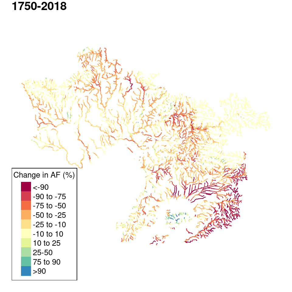
The difference between 1750 AF estimates and 2018 estimates (Figure 7.8) suggests that for most contemporary forested areas (and grassland areas in the west of Melbourne) the 1750 estimates are a good match for 2018 estimates (areas with between -10 and 10% difference), although. It also shows the substantial loss of forest cover across the region, most notably in the south-east (orange-red lines). A few small areas suggest an increase in forest cover (green-blue lines). For French Island, Nearmap data was not available, and I have used 2006 forest data, which overestimated tree cover for heathland areas. Care should be taken using contemporary estimates for French Island until new forest cover data is received. For other areas, it is possible that the forests have become denser since 1750: for instance the woodlands of Pyrites Creek downstream of Merrimu Reservoir had denser cover in 2018 than was assumed for their 1750 status of grassy and buloak woodland with riparian shrubland.
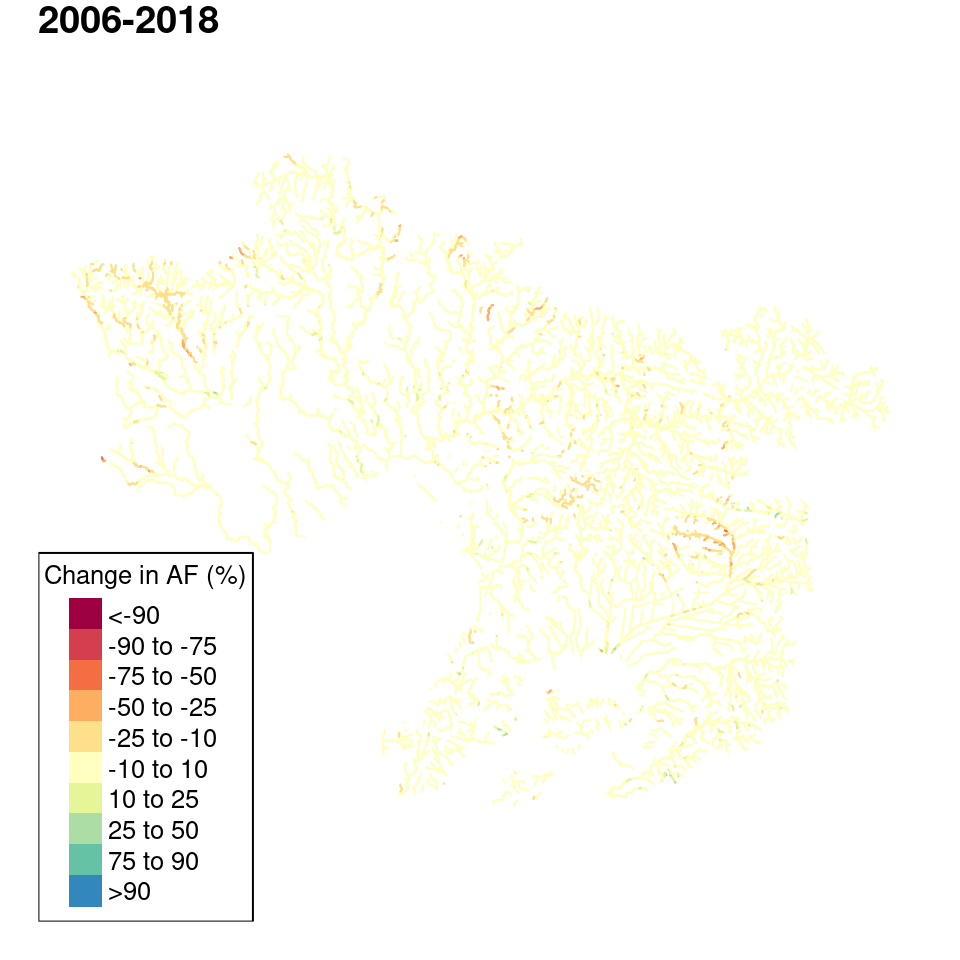
The difference between 2006 AF estimates and 2018 estimates (Figure 7.9) suggest that tree cover in forests tended to be slightly overestimated for the 2006 data. This was expected as upslope forests in the 2006 data were represented as 100% canopy cover, while the Nearmap data more realistically quantifies canopy gaps. Note that areas of complete agreement between 2006 and 2018 (e.g. the upper Yarra catchment and French Island) are a result of the 2006 data being used to fill gaps in the later data. Lines with positive growth between these two years (green lines) are likely to be true representations of reafforestation over the period.
For much of the regions there is little difference between 2018 AF estimates and 2022 estimates (Figure 7.10). In version 1.3 of the database, there were large areas of AF decrease between 2018 and 2022, but much of these differences were a result of underestimations of tree cover in the 2018 Nearmap data. These differences have been corrected for version 1.3.1 (see Appendix E). The remaining decreases in AF between the years are the result of real losses of forest mainly because of 2019 storm damage (perhaps with subsequent clearing, in the Wombat Forest in the north-west, the Cobaw Ranges in the north, and the Dandenong Ranges in the inner east) and logging (in the north-west ranges and Bunyip Ranges in the southeast) for the Dandenong Ranges, the imagery suggests a thinning of forest cover over that time. There are also a few isolated reaches suggesting a small increase in tree cover over that time (mainly in the west), and the imagery for those areas do show some tree growth over that time.

The total area of gridcells in some subcatchments (
area_r_m2in the subc_env table) differs slightly from its subcatchment area (scareain the subcs table), which was calculated from polygon areas, some of which were edited to better match the stream lines. The sum of all upstreamarea_r_m2upstream iscat_area_m2_rin the cat_env table, and the sum of all upstreamscarea(divided by 1000) iscarea_km2in the subcs table (see Chapter 4).↩︎