# In this example the gpkg files are in a subfolder of the working directory
mwstr_dir <- "mwstr_v13/"
# Create a sqlite connection to the database and to the cats layer
db_m <- RSQLite::dbConnect(drv = RSQLite::SQLite(),
paste0(mwstr_dir,"mwstr_v1.3.1.gpkg"))
db_c <- RSQLite::dbConnect(drv = RSQLite::SQLite(),
paste0(mwstr_dir,"mwstr_cats_v1.3.gpkg"))
# Retrieve site and nextds fields for all subcs and convert to an igraph
# object for rapid network calculations
subcs <- RSQLite::dbGetQuery(db_m,"SELECT site, nextds FROM subcs;")
subcs <- apply(subcs, 2, as.character)
subcs_ig <- igraph::graph_from_data_frame(subcs)
# Retrieve details for Riddells Creek
riddells_ck <- RSQLite::dbGetQuery(db_m,
"SELECT * FROM stream_names WHERE SUBSTR(str_nm,1,7) = 'RIDDELL';")
# Inspecting the object riddells_ck reveals strcode for Riddells Creek is
# RID, and terminal reach is 11580
# Retrieve all reaches upstream of Riddells Creek's terminal reach
x <- subcs[igraph::subcomponent(subcs_ig, "11580", "in"),1]
rid_network <- sf::st_read(db_m, query = paste0("SELECT * FROM streams ",
"WHERE site IN (",paste(x, collapse = ", "), ");"))
# Retrieve Riddells Creek mainstem
rid_ms <- sf::st_read(db_m, query =
"SELECT * FROM streams WHERE SUBSTR(reach,1,3) = 'RID';")
# Retrieve catchment boundary for terminal reach of Riddells Creek
rid_cat <- sf::st_read(db_c,
query = "SELECT * FROM cats WHERE site = 11580;")
# Disconnect database connections
RSQLite::dbDisconnect(db_m); RSQLite::dbDisconnect(db_c)
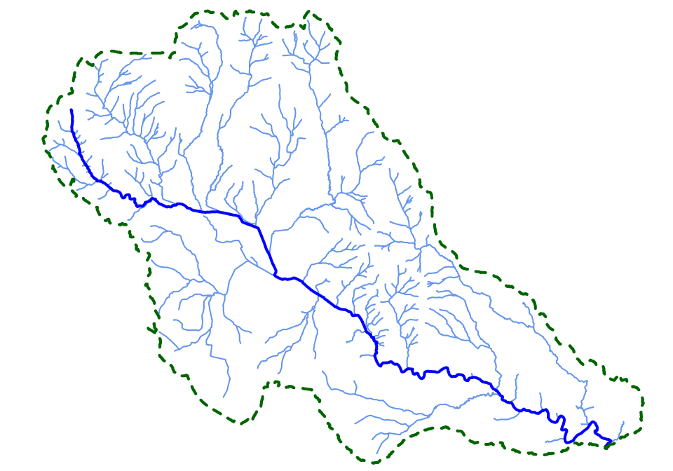
# Plot the stream, its tribs and its catchment
par(mar = c(0,0,0,0))
plot(rid_network$geom, col = "cornflowerblue")
plot(rid_ms$geom, col = "blue", lwd = 2, add = TRUE)
plot(rid_cat$geom, border = "darkgreen", lwd = 2, lty = 2, add = TRUE)The Melbourne Stream Network User’s Manual (Walsh 2023) provides full technical details on the provenance of the data and its usage, available here.
This page provides a brief overview of the structure of the database, how to access and use the data, and a list of useful links to sections of the manual
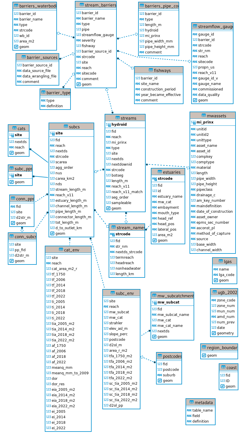
Database structure
The following is a table-relationships diagram derived from the postgreSQL database.
An example of using the data
While each vector table can be loaded individually into GIS software from the gpkg file, information can often be more efficiently extracted from the gpkg file using SQL queries. Here are a few examples of such an approach using R.
Example code for extracting information from the database selectively to rapidly produce a map of all reaches upstream of a point of interest (in this case the terminal reach of Riddells Creek in the Macedon Ranges). These steps are compiled into the helper function plot_allus() (see Walsh (2023) Chapter 4)
Useful links to manual sections
The intuitive unique stream names and codes, and reach codes are a central element of the network.
The logic of the chosen stream names is explained in section 3.5 of the manual.
The unique 3-character stream code (
strcode) for each stream can be looked up quickly using the stream selector in the app (as well as in the stream_names table of the database).The reach code (
reach) convention is explained in section 4.3.
The manual includes advice on reading and manipulating the data, including example code snippets.
Example code/instructions for:
Reading the data into R — Appendix C.1.1 (see also above)
Reading the data in QGIS or ArcGIS — Appendix C.1.2
Compiling the data into a postgreSQL database — Appendix C.2
Calculating upstream catchment statistics for the entire network given sub-catchment statistics — Section 4.2
Calculating distances and numbers of barriers between given reaches in the network — Section 10.4
Example code for plotting maps of:
study sites, and their catchments and streams — Section 3.2
the streams and catchment upstream of a given reach, with optional base maps – Section 4.4
the stream network coloured by selected environmental variables —Sections 5.9-11
References
Walsh, C J. 2023. “Melbourne Water Stream Network. Version 1.3. Melbourne Water Research Practice Partnership Technical Report 19.4d.” Report. School of Agriculture, Food and Ecosystem Sciences, The University of Melbourne. https://tools.thewerg.unimelb.edu.au/mwstr_manual/.