db_m <- RSQLite::dbConnect(drv = RSQLite::SQLite(),
                                          "data/mwbugs_db_v2.1_public.gpkg")
The Melbourne Water Macroinvertebrate Dabase User’s Manual (Walsh 2025) provides full technical details on the provenance of the data and its usage, available here.
This page provides a brief overview of the structure of the database, how to access and use the data, and a list of useful links to sections of the manual
Database structure
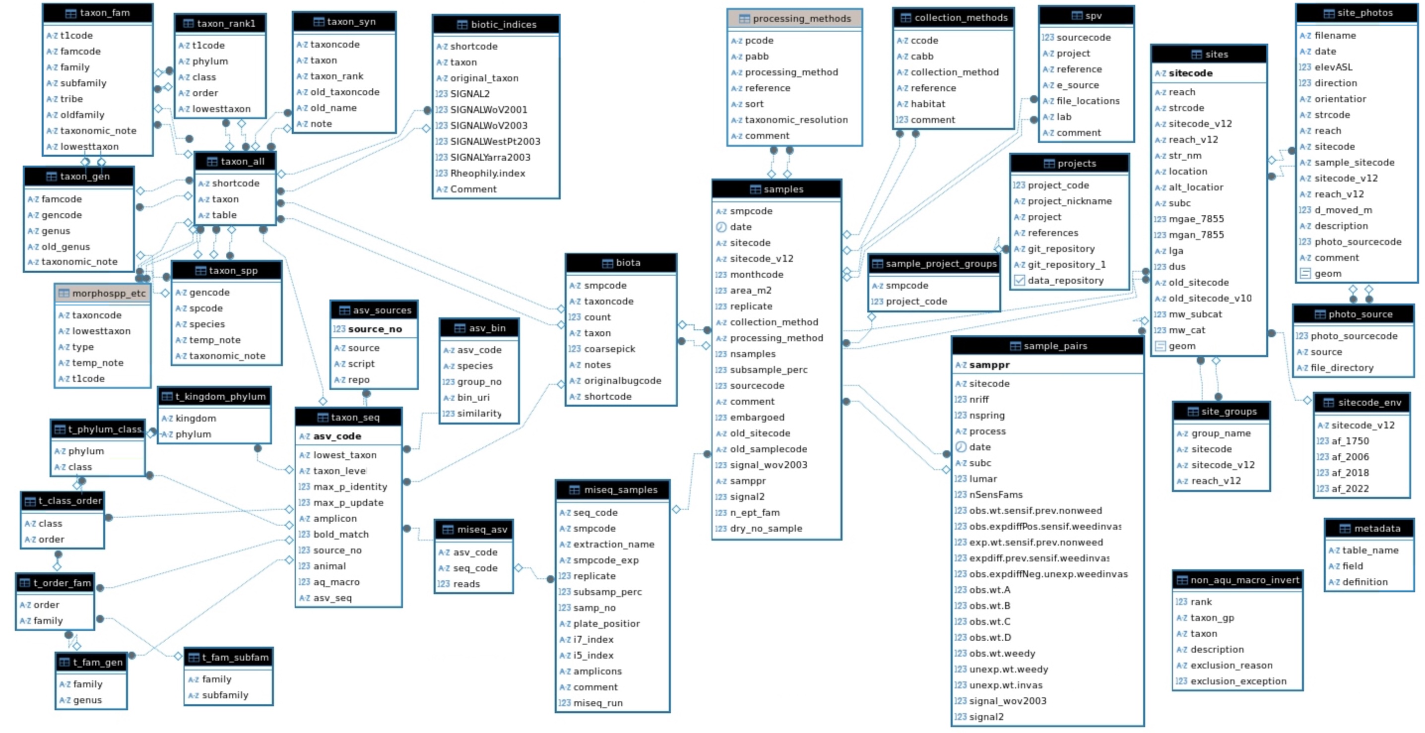
The following is a table-relationships diagram derived from the postgreSQL database.

Accessing the data
If you are unfamiliar with manipulating related tables using SQL or in R (or another code-based program), you may find downloading subsets of the data from the data explorer app the easiest approach to accessing the data.
To access the full database, see Section 2.2 of the database user’s manual.
Once you have access to the database, you need to create a connection to it to read its tables. Here is an example of creating a connection to the gpkg version of the database in R, having downloaded it to a subfolder data
of the working directory.
The two spatial tables in the database (sites and site_photos) can be loaded individually into GIS software from the gpkg file. However, their data and that of the non-saptial tables can be more efficiently extracted from the gpkg file using SQL queries, or through equivalent manipulations in R. The database is small enough that all its tables can be quickly loaded into an R environment using a single command load_all_mwbugs_tables() from bug_database_functions.R.
source(paste0("https://tools.thewerg.unimelb.edu.au/mwbugs/data/",
"bug_database_functions.R"))load_all_mwbugs_tables(db_m)
# Always remember to disconnect from database once data is accessed
DBI::dbDisconnect(db_m)Having connected to the database, you can find examples of how to use the data in the user’s manual:
Extracting data tables by project Section 6.3.3
Compiling a taxon-by-sample matrix for a subset of samples Section 8.1
Creating a map of occurrences of a given taxon Secton 8.2
Plotting a time series of LUMaR scores Section 4.2
Other useful links to manual sections
More information on accessing the database are in section 2.2
The logic of the sitecode conventions and their links to the stream network database are detailed in Chapter 3
Sample code (smpcode) logic, including how to convert monthcodes into dates and how to translate the trailing characters of smpcodes into sample collection and processing methods, is detailed in Section 4.1
Instructions on preparing a sites table, including automatically deriving standard sitecodes given point locations, are in Section 7.1.
The manual includes advice on reading and manipulating the data, including example code snippets.
Example code/instructions for:
Reading the data into R - Section 2.2 and Appendix B section B1.1.
Reding the data in QGIS or ArcGIS - Appendix B section B1.2
Compiling the data intp a postgreSQL database - Appendix B section B2
Compiling a hierarchical taxonomy table given a vector of taxoncodes - Section 5.3
Compiling a hierarchical taxonomy table given a vector of DNA sequences - Section 6.1.1