4  Samples and sample_pairs tables

4.1 Samples

As of this report’s publication, the samples table contained details of 9,320 from 1,010 sites.

The primary field of the samples table is smpcode: a unique code comprising hyphen-separated monthcode, sitecode, replicate number, and a two-character code indicating collection and processing methods (ccode and pcode: see below).

For instance smpcode 072-GRD-5879-0-1-BH signifies a sample collected in month 072 (Dec 1995) from Gardiners Creek (GRD) at Solway Street Ashburton, where its catchment area is 5.879 km², zero indicating that the site is at the bottom of the reach). The sample is a single sample (or possibly the first replicate taken at the site) from a riffle using a standard bioassessment kick net, lab-sorted to a 300-count subsample, identified to lowest taxon. The conventions for these calculations are explained below.

sitecode is matched to the unique sitecodes in the sites table: see the section above for an explanation of the sitecode logic. The month code is a three-digit integer indicating the number of months since December 1989 (e.g. Jan 1990 = 01, Jan 1992 = 25). The date that the sample was taken is recorded in the date field. monthcodes can be calculated in R from dates and translated back into dates using two functions in the file “bug_database_functions.R”.

# translate a date into a monthcode
calcMonthDate(lubridate::ymd("1995-12-10"))

[1] 72

# translate a monthcode to a date
calcMonthNo(72)

[1] "Dec 1995"

The replicate field is used to distinguish samples taken from the same habitat using the same collection method in the same month. For most samples there are no such replicates, and replicate = 1.

Collection method distinguishes both the collection method and the habitat sampled. Each collection method is represented in the smpcode by a single character (ccode). The collection_method field links to the collection_methods table, which details all collection methods recorded in the database (with potential for augmentation with other methods as the database grows: Table 4.1).

Table 4.1: The collection_methods table. ccode is used to identify collection methods in samplecodes. The entries in reference refer to bibtex entries in the associated reference.bib.

ccode	cabb	collection_method	reference	habitat
A	RBA-E-	RBA edge (sweep)	epa_vic_2003	edge
B	RBA-R-	RBA riffle (kick)	epa_vic_2003	riffle
C	RBA-C-	RBA composite (sweep-kick)	epa_vic_2003	edge and riffle
D	RBA-C-	RBA edge-riffle combined	epa_vic_2003	edge and riffle
E	RBA-E-	RBA two edges combined	epa_vic_2003	edge
F	H-B-	Hess sampler, benthos	hess_1941	benthos
G	H-B-	micro-Hess sampler, benthos		benthos
H	A-B-	airlift, benthos, single sample	hellawell_1978	benthos
I	S-W-	snag bag, large woody debris, single sample	growns_etal_1999	large wooody debris
J	A-M-	airlift, benthos, samples combined	hellawell_1978	benthos
K	S-W-	snag bag, large woody debris, samples combined	growns_etal_1999	large woody debris
L	B-B-	Boulton suction sampler, benthos, single sample	boulton_1985	benthos
M	B-B-	Boulton suction sampler, benthos, samples combined	boulton_1985	benthos
N	S-W-	sweep and jab over natural large woody debris	ghd_2013	large woody debris
O	S-W-	sweep and jab over artificial large woody debris	ghd_2013	large woody debris

Processing method distinguishes both the method used to sort the sample following collection and the taxonomic resolution to which the sample was identified. Each processing method is represented in the samplecode by a single character (pcode). The processing_method field links to the processing_methods table, which details all processing methods recorded in the database (with tentative, as yet unused fields for anticipated new data arising from DNA methods: Table 4.2).

Table 4.2: The processing_methods table. pcode is used to identify processing methods in samplecodes. The entries in reference refer to bibtex entries in the associated reference.bib.

pcode	pabb	processing_method	reference	sort	taxonomic_resolution
A	F-F	30-min field-sort, ID to family	epa_vic_2003	field	family
B	L-F	lab-subsample to 200, ID to family	walsh_1997	lab	family
C	L-F	lab-subsample to 300, ID to family	walsh_1997	lab	family
D	L-F	lab-subsample to 400, ID to family	walsh_1997	lab	family
C	L-G	lab-subsample to 200, ID to genus	walsh_1997	lab	genus
E	L-G	lab-subsample to 400, ID to genus	walsh_etal_2007	lab	genus
F	F-L	30-min field-sort, ID to lowest taxon	epa_vic_2003	field	lowest
G	L-L	lab-subsample to 200, ID to lowest taxon	walsh_1997	lab	lowest
H	L-L	lab-subsample to 300, ID to lowest taxon	walsh_1997	lab	lowest
I	L-F	lab complete sort, ID to family		lab	family
K	L-L	lab complete sort, ID to lowest taxon		lab	lowest
R	R-F	residue of subsampling to family
S	R-L	residue of subsampling to lowest taxon
N	N	no sample taken
O	L-G	lab-subsample to 300, ID to genus		lab	genus
J	L-G	lab complete sort, ID to genus		lab	genus
L	L-D	lab-subsample to 300, DNA barcoding ID to species	carew_etal_2018	lab	species
M	L-D	bulk processing of 2 combined samples, DNA barcoding ID to species	carew_etal_2023	lab	species

For quantitative collection methods, the area sampled is recorded in the samples table field area_m2. For some quantitative sampling methods, replicate samples were combined before processing. In such cases (e.g. the airlift and snag-bag samples of the Yarra Ecological study, C. J. Walsh et al. 2007), the number of sample units in the combined sample is recorded in the field nsamples, and the area_m2 field records the total area sampled by all sample units. For samples that have been subsampled, the percentage subsample is recorded in the subsample_perc table. It is important to note that the counts recorded in the biota table are raw counts: total abundance in subsampled samples can be approximately estimated as count*100/subsample_perc. However, a better way to use count and subsample_perc data is to model subsample error in any statistical model of taxon counts: see C. J. Walsh et al. (2023) for an example.

Both the collection_methods and processing_methods tables include a more intuitive abbreviation field (cabb and pabb, respectively). These abbreviations are used by the web interface (see below) to summarise the methods used for collections of samples.

The sourcecode field links to the field of the same name in sample_provenance table. Samples, as much as possible, have been allocated to a single project which commissioned their collection, and the sample_provenance table lists relevant details about that project including the name of the project, publications arising from each project (bibtex citations linked to mwbugs.bib¹), information on the source and format of the data as supplied before it was entered into the database, and the laboratory that collected and processed each project. For some sets of samples, allocation to individual projects was not simple. For instance, samples that have been allocated to Phase III of the Little Stringybark Creek project (sourcecode 3), were also collected as part of MW’s annual monitoring program. In such cases projects were allocated on the basis of the most likely avenue for publication using the data.

Data for some samples will not be included in the publicly available version of the data if preparation of publications using the data is in progress. Such samples will be identified in the samples table using the embargoed field. If the sample data are being held back for publication embargoed = 1.

The fields old_sitecode and old_samplecode are included in the samples table to maintain a link with old versions of the database.

4.2 Biotic metrics and the sample_pairs table

The samples table contains three metrics summarizing macroinvertebrate assemblage composition in each sample: SIGNAL2 [signal2; Chessman (2003)], and SIGNAL SEPP Waters of Victoria [signal_wov2003; EPA Victoria (2004)], and Number of EPT families (n_ept_fam).

samppr codes in the samples table group pairs of samples collected from the same site on the same day, or in some cases in consecutive seasons. The combined family accurrences in each samppr were used to calculate the range of metrics calculated by the melbstreambiota R package (C. Walsh C J 2019) and are compiled in the sample_pairs table. LUMAR is a macroinvertebrate metric [walsh_2023a] that is used to assess stream condition by Melbourne Water’s 2018 Healthy Waterways Strategy. Figure 4.1 uses the lumar_plot() function from bug_database_functions.R (see the data downloads page of the database website) to plot a time series of LUMaR scores for the long-term monitoring site on the Yarra River at Templestowe, showing a decline in condition associated with increased urban development in its catchment.

# Find reach of Yarra at Fitzsimons Lane, Templestowe
site_yar <- sites[sites$strcode == "YAR" & grepl("Fitzsimons", sites$location),]
#lumarPlot function in bug_database_functions.R 
lumar_plot(site_yar$sitecode)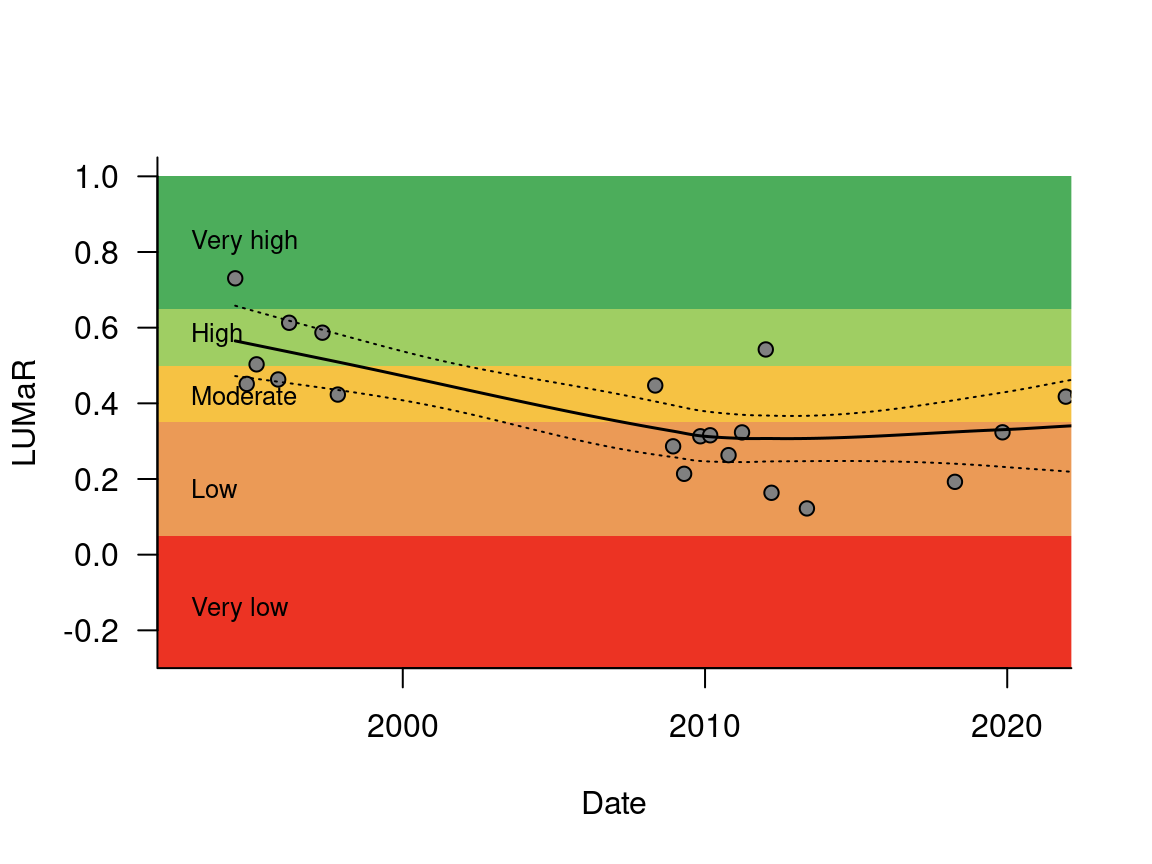 

Figure 4.1: Trend in LUMaR score over the period of record in the macroinvertebrate database for site YAR-275352-4, Fitzsimons Lane- Templestowe, drawn from the sample_pairs table. The solid line is a loess curve fit to the data (span 1, degree 1), with 95% confidence bounds as dashed lines.

Chessman, B C. 2003. “New Sensitivity Grades for Australian River Macroinvertebrates.” Journal Article. Marine and Freshwater Research 54 (2): 95–103.

EPA Victoria. 2004. “Biological Objectives for Rivers and Streams–Ecosystem Protection.” Report 793.2. Environment Protection Authority Victoria.

Walsh, C J, K A Waller, J Gehling, and R Mac Nally. 2007. “Riverine Invertebrate Assemblages Are Degraded More by Catchment Urbanization Than by Riparian Deforestation.” Freshwater Biology 52: 574–87. http://citeseerx.ist.psu.edu/viewdoc/download?doi=10.1.1.631.6082&rep=rep1&type=pdf.

Walsh, C J, J A Webb, Gwinn D C, and P F Breen. 2023. “Constructed Rock Riffles Increase Habitat Heterogeneity but Not Biodiversity in Streams Constrained by Urban Impacts.” Ecosphere, in review.

Walsh, Chee, C J. 2019. “Assessing and Understanding in-Stream Habitat Suitability for Invertebrate Families, Fish Species and Platypus of the Melbourne Region with the Melbstreambiota Package (Version 0.1.2).” https://osf.io/v2tda.

---

1. mwbugs.bib is available from the database download page of the database web site.