db_m <- DBI::dbConnect(drv = RSQLite::SQLite(),
paste0(wd,"mwbugs/mwbugs_public.gpkg"))2 Database structure and how to access it
2.1 Database structure
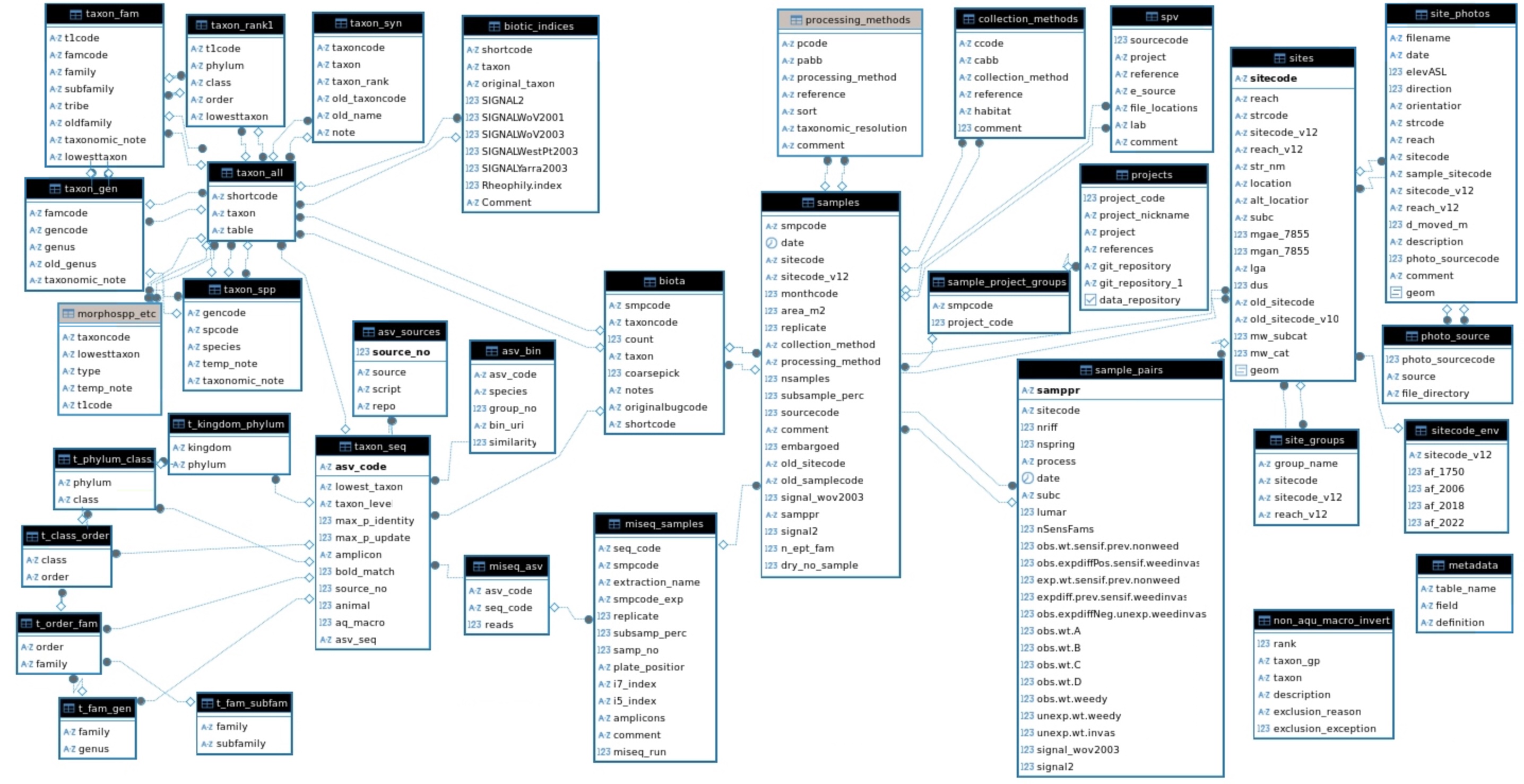
Three tables constitute the core of the database (Figure 2.1):
The sites table lists every sampled site, identified by a unique
sitecode;The samples table lists every sample taken at each site, identified by a unique
samplecode;The biota table lists every taxon and
count(number identified in each potentialy sub-sampled sample).
Two additional tables are used to organize differences in collection methods and processing methods among samples, and a third is used to group samples by the primary project for which they were collected, with links to project reports (Figure 2.1). Earlier versions of the database used a single taxonomic table with unique taxoncodes to link to the biota table. We use a different approach to taxonomy in this version of the database, as detailed in (Section 5.2).
Since version 2, an additional spatial table, site_photos, and an associated photo_sources table have been added as a record of sampling reaches, and for confirmation of their locations (see Chapter 3). The addition of DNA-based data in 2025 resulted in the addition of many tables centring around taxon_seq, miseq_asv, and miseq_samples that store DNA sequence data and their taxonomic identities for aggregation to species-sample records that have been added to the biota table (see Chapter 6)
2.2 Accessing the database tables
You can download subsets of the database using the data explorer app.
You can download the whole database (as a SQLite geopackage file) or just the taxonomic tables (as an excel file) on the data download tab of the database website. (Or, if you are on the unimelb network, you can access the master postgreSQL version of the database: contact Chris Walsh for further information.)
You can convert the geopackage tables into a postgreSQL database, using the instructions in Appendix B.
Regardless of the database format (SQLite, postgreSQL or other relational database software), to access the data in R, you need to create a connection to the database. If you have saved the downloaded geopackage file to a subdirectory of the working directory (‘wd’) named ‘mwbugs’, you can connect to it using the following commands.
(See Appendix B for the equivalent command for connecting to a postgreSQL database.)
To then read all tables into the R environmental with a single command,
source(paste0("https://tools.thewerg.unimelb.edu.au/mwbugs/data/",
"bug_database_functions.R"))load_all_mwbugs_tables(db_m)
# Always remember to disconnect from database once data is accessed
DBI::dbDisconnect(db_m)Alternatively, you can read single tables or select subsets and combinations of one or more tables using SQL queries. See Appendix B for further instructions.